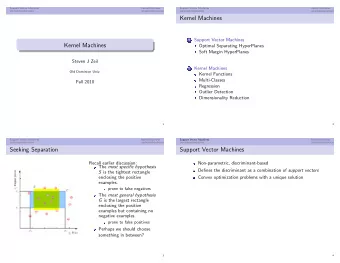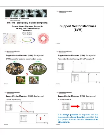
[PPT] - SUPPORT VECTOR MACHINES FOR BANKRUPTCY ANALYSIS Wolfgang H ARDLE 2 PowerPoint Presentation

SLIDE 1

1

SUPPORT VECTOR MACHINES FOR BANKRUPTCY ANALYSIS

Wolfgang H¨ ARDLE 2 Rouslan MORO 1,2 Dorothea SCH¨ AFER 1

1 Deutsches Institut f¨

ur Wirtschafts- forschung (DIW)

2 Center for Applied Statistics and Eco-

nomics (CASE), Humboldt-Universit¨ at zu Berlin

Corporate Bankruptcy Prediction with SVMs

SLIDE 2

Motivation 2

Linear Discriminant Analysis

Fisher (1936); company scoring: Beaver (1966), Altman (1968) Z-score: Zi = a1xi1 + a2xi2 + ... + adxid = a⊤xi, where xi = (xi1, ..., xid)⊤ ∈ Rd are financial ratios for the i-th company. The classification rule: successful company: Zi ≥ z failure: Zi < z

Corporate Bankruptcy Prediction with SVMs

SLIDE 3

Motivation 3

Linear Discriminant Analysis

X

1

X

2

Surviving companies

x

Failing

companies

x x x x x x x x x x x x x x x x x x x x x x x x x x x x x

x

x x x

?

Corporate Bankruptcy Prediction with SVMs

SLIDE 4

Motivation 4

Linear Discriminant Analysis

Z Distribution density

Surviving companies Failing companies Score

Corporate Bankruptcy Prediction with SVMs

SLIDE 5

Motivation 5

Company Data: Probability of Default

Source: Falkenstein et al. (2000)

Corporate Bankruptcy Prediction with SVMs

SLIDE 6

Motivation 6

RiskCalc Private Model

Moody’s default model for private firms A semi-parametric model based on the probit regression E[yi|xi] = Φ{a0 +

d

j=1

ajfj(xij)} fj are estimated non-parametrically on univariate models

Corporate Bankruptcy Prediction with SVMs

SLIDE 7

Motivation 7

Linearly Non-separable Classification Problem

X

1

X

2

Surviving companies

x x x x x x x x x x x x x x x x x x x x x x x

o
x

x x x x x x

Failing companies

x 3 1 2

x

Corporate Bankruptcy Prediction with SVMs

SLIDE 8

Outline of the Talk 8

Outline

1. Motivation
2. Support Vector Machines and their Properties
3. Expected Risk vs. Empirical Risk Minimization
4. Realization of an SVM
5. Non-linear Case
6. Company Classification and Rating with SVMs

Corporate Bankruptcy Prediction with SVMs

SLIDE 9

Support Vector Machines and Their Properties 9

Support Vector Machines (SVMs)

SVMs are a group of methods for classification (and regression) that make use of classifiers providing “high margin”. ⊡ SVMs possess a flexible structure which is not chosen a priori ⊡ The properties of SVMs can be derived from statistical learning theory ⊡ SVMs do not rely on asymptotic properties; they are especially useful when d/n is big, i.e. in most practically significant cases ⊡ SVMs give a unique solution and outperform Neural Networks

Corporate Bankruptcy Prediction with SVMs

SLIDE 10

Support Vector Machines and Their Properties 10

Classification Problem

Training set: {(xi, yi)}n

i=1 with the distribution P(xi, yi).

Find the class y of a new object x using the classifier f : Rd → {+1; −1}, such that the expected risk R(f) is minimal. xi ∈ Rd is the vector of the i-th object characteristics; yi ∈ {−1; +1} or {0; 1} is the class of the i-th object.

Regression Problem

Setup as for the classification problem but: y ∈ R

Corporate Bankruptcy Prediction with SVMs

SLIDE 11

Expected Risk vs. Empirical Risk Minimization 11

Expected Risk Minimization

Expected risk R(f) = 1 2|f(x) − y|dP(x, y) = EP (x,y)[L(x, y)] is minimized wrt f: fopt = arg min

f∈F R(f)

L(x, y) = 1 2 |f(x) − y| =    0, if classification is correct, 1, if classification is wrong. F is an a priori defined set of (non)linear classifier functions

Corporate Bankruptcy Prediction with SVMs

SLIDE 12

Expected Risk vs. Empirical Risk Minimization 12

Empirical Risk Minimization

In practice P(x, y) is usually unknown: use Empirical Risk ˆ R(f) = 1 n

n

i=1

1 2|f(xi) − yi| Minimization (ERM) over the training set {(xi, yi)}n

i=1

ˆ fn = arg min

f∈F

ˆ R(f)

Corporate Bankruptcy Prediction with SVMs

SLIDE 13

Expected Risk vs. Empirical Risk Minimization 13

Empirical Risk vs. Expected Risk

Function class Risk f f

pt

R R

(f)

f

n

ˆ

R

(f)

ˆ

R

ˆ

Corporate Bankruptcy Prediction with SVMs

SLIDE 14

Expected Risk vs. Empirical Risk Minimization 14

Convergence

From the law of large numbers lim

n→∞

ˆ R(f) = R(f) In addition ERM satisfies lim

n→∞ min f∈F

ˆ R(f) = min

f∈F R(f)

if “F is not too big”.

Corporate Bankruptcy Prediction with SVMs

SLIDE 15

Expected Risk vs. Empirical Risk Minimization 15

Vapnik-Chervonenkis (VC) Bound

Basic result of Statistical Learning Theory (for linear classifiers): R(f) ≤ ˆ R(f) + φ h n, ln(η) n

where the bound holds with probability 1 − η and

φ h n, ln(η) n

=
h(ln 2n

h + 1) − ln( η 4)

n

Corporate Bankruptcy Prediction with SVMs

SLIDE 16

Expected Risk vs. Empirical Risk Minimization 16

Structural Risk Minimization

Structural Risk Minimization – search for the model structure Sh, Sh1 ⊆ Sh2 ⊆ . . . ⊆ Sh ⊆ . . . ⊆ Shk ⊆ F, such that f ∈ Sh minimizes the expected risk upper bound. h is VC dimension. Sh is a set of classifier functions with the same complexity described by h, e.g. P(1) ⊆ P(2) ⊆ P(3) ⊆ . . . ⊆ F, where P(i) are polynomials of degree i. The functional class F is given a priori

Corporate Bankruptcy Prediction with SVMs

SLIDE 17

Expected Risk vs. Empirical Risk Minimization 17

Vapnik-Chervonenkis (VC) Dimension

Definition. h is VC dimension of a set of functions if there exists a set
f points {xi}h

i=1 such that these points can be separated in all 2h

possible configurations, and no set {xi}q

i=1 exists where q > h satisfies

this property. Example 1. The functions f = A sin θx have an infinite VC dimension. Example 2. Three points on a plane can be shattered by a set of linear indicator functions in 2h = 23 = 8 ways (whereas 4 points cannot be shattered in 2q = 24 = 16 ways). The VC dimension equals h = 3. Example 3. The VC dimension of f = {Hyperplane ∈ Rd} is h = d + 1.

Corporate Bankruptcy Prediction with SVMs

SLIDE 18

Expected Risk vs. Empirical Risk Minimization 18

VC Dimension (d=2, h=3)

Corporate Bankruptcy Prediction with SVMs

SLIDE 19

Realization of the SVM 19

Linearly Separable Case

The training set: {(xi, yi)}n

i=1, yi = {+1; −1}, xi ∈ Rd. Find the

classifier with the highest “margin” – the gap between parallel hyperplanes separating two classes where the vectors of neither class can

lie. Margin maximization minimizes the VC dimension.
x

x x x x x x x x

x
Corporate Bankruptcy Prediction with SVMs

SLIDE 20

Realization of the SVM 20

Linear SVMs. Separable Case

The margin is d+ + d− = 2/w. To maximize it minimize the Euclidean norm w subject to the constraint (1).

b
|

w |

x
x

x

x x x x x

x

w x

Tw+b=0

x

1

x

2

margin d

- d

+

x

Tw+b=1

x

Tw+b=-1

Corporate Bankruptcy Prediction with SVMs

SLIDE 21

Realization of the SVM 21

Let x⊤w + b = 0 be a separating hyperplane. Then d+ (d−) will be the shortest distance to the closest objects from the classes +1 (−1). x⊤

i w + b ≥ +1 for yi = +1

x⊤

i w + b ≤ −1 for yi = −1

combine them into one constraint yi(x⊤

i w + b) − 1 ≥ 0

i = 1, 2, ..., n (1) The canonical hyperplanes x⊤

i w + b = ±1 are parallel and the distance

between each of them and the separating hyperplane is d+ = d− = 1/w.

Corporate Bankruptcy Prediction with SVMs

SLIDE 22

Realization of the SVM 22

The Lagrangian Formulation

The Lagrangian for the primal problem LP = 1 2w2 −

n

i=1

αi{yi(x⊤

i w + b) − 1}

The Karush-Kuhn-Tucker (KKT) Conditions

∂LP ∂wk = 0

⇔ n

i=1 αiyixik = 0

k = 1, ..., d

∂LP ∂b = 0

⇔ n

i=1 αiyi = 0

yi(x⊤

i w + b) − 1 ≥ 0

i = 1, ..., n αi ≥ 0 αi{yi(x⊤

i w + b) − 1} = 0 Corporate Bankruptcy Prediction with SVMs

SLIDE 23

Realization of the SVM 23

Substitute the KKT conditions into LP and obtain the Lagrangian for the dual problem LD =

n

i=1

αi − 1 2

n

i=1

n

j=1

αiαjyiyjx⊤

i xj

The primal and dual problems are min

wk,b max αi LP

max

αi LD

s.t. αi ≥ 0

n

i=1

αiyi = 0 Since the optimization problem is convex the dual and primal formulations give the same solution.

Corporate Bankruptcy Prediction with SVMs

SLIDE 24

Realization of the SVM 24

The Classification Stage

The classification rule is: g(x) = sign(x⊤w + b) where w = n

i=1 αiyixi

b = 1

2(x+ + x−)⊤w

x+ and x− are any support vectors from each class αi = arg max

αi LD

subject to the constraint yi(x⊤

i w + b) − 1 ≥ 0

i = 1, 2, ..., n.

Corporate Bankruptcy Prediction with SVMs

SLIDE 25

Realization of the SVM 25

Linear SVMs. Non-separable Case

In the non-separable case it is impossible to separate the data points with hyperplanes without an error.

x

x x x x x x x x

x
x

Corporate Bankruptcy Prediction with SVMs

SLIDE 26

Realization of the SVM 26

Linear SVM. Non-separable Case

Corporate Bankruptcy Prediction with SVMs

SLIDE 27

Realization of the SVM 27

The problem can be solved by introducing positive slack variables {ξi}n

i=1 into the constraints

x⊤

i w + b

≥ 1 − ξi for yi = 1 x⊤

i w + b

≤ −1 + ξi for yi = −1 ξi ≥ ∀i If an error occurs, ξi > 1. The objective function: 1 2w2 + C

n

i=1

ξi where C (“capacity”) controls the tolerance to errors on the training set. Under such a formulation the problem is convex

Corporate Bankruptcy Prediction with SVMs

SLIDE 28

Realization of the SVM 28

The Lagrangian Formulation

The Lagrangian for the primal problem for ν = 1: LP = 1 2w2 + C

n

i=1

ξi −

n

i=1

αi{yi(x⊤

i w + b) − 1 + ξi} − n

i=1

ξiµi The primal problem: min

wk,b,ξi max αi,µi LP Corporate Bankruptcy Prediction with SVMs

SLIDE 29

Realization of the SVM 29

The KKT Conditions

∂LP ∂wk = 0

⇔ wk = n

i=1 αiyixik

k = 1, ..., d

∂LP ∂b = 0

⇔ n

i=1 αiyi = 0 ∂LP ∂ξi = 0

⇔ C − αi − µi = 0 yi(x⊤

i w + b) − 1 + ξi ≥ 0

ξi ≥ 0 αi ≥ 0 µi ≥ 0 αi{yi(x⊤

i w + b) − 1 + ξi} = 0

µiξi = 0

Corporate Bankruptcy Prediction with SVMs

SLIDE 30

Realization of the SVM 30

The dual Lagrangian does not contain ξi or their Lagrange multipliers LD =

n

i=1

αi − 1 2

n

i=1

n

j=1

αiαjyiyjx⊤

i xj

(2) The dual problem is max

αi LD

subject to 0 ≤ αi ≤ C

n

i=1

αiyi = 0

Corporate Bankruptcy Prediction with SVMs

SLIDE 31

Non-linear Case 31

Non-linear SVMs

Map the data to a Hilbert space H and perform classification there Ψ : Rd → H Note, that in the Lagrangian formulation (2) the training data appear

nly in the form of dot products x⊤

i xj, which can be mapped to

Ψ(xi)⊤Ψ(xj). If a kernel function K exists such that K(xi, xj) = Ψ(xi)⊤Ψ(xj), then we can use K without knowing Ψ explicitly

Corporate Bankruptcy Prediction with SVMs

SLIDE 32

Non-linear Case 32

Mapping into the Feature Space. Example

R2 → R3, Ψ(x1, x2) = (x2

1,

√ 2x1x2, x2

2)⊤,

K(xi, xj) = (x⊤

i xj)2 Data Space Feature Space

x x x x x x x x x x x x x x x x x x x x x x x x x x x x x

o
o
x

x x x x

Corporate Bankruptcy Prediction with SVMs

SLIDE 33

Non-linear Case 33

Mercer’s Condition (1909)

A necessary and sufficient condition for a symmetric function K(xi, xj) to be a kernel is that it must be positive definite, i.e. for any x1, ..., xn ∈ Rd and any λ1, ..., λn ∈ R the function K must satisfy:

n

i=1

n

j=1

λiλjK(xi, xj) ≥ 0 Examples of kernel functions: K(xi, xj) = e−(xi−xj)⊤Σ−1(xi−xj)/2 anisotropic Gaussian kernel K(xi, xj) = (x⊤

i xj + 1)p

polynomial kernel K(xi, xj) = tanh(kx⊤

i xj − δ)

hyperbolic tangent kernel

Corporate Bankruptcy Prediction with SVMs

SLIDE 34

Non-linear Case 34

Classes of Kernels

Stationary kernel is a kernel which is translation invariant: K(xi, xj) = KS(xi − xj) Isotropic (homogeneous) kernel is one which depends only on the distance between two data points: K(xi, xj) = KI(xi − xj) Local stationary kernel is a kernel of the form: K(xi, xj) = K1(xi + xj 2 )K2(xi − xj) where K1 is a non-negative function, K2 is a stationary kernel.

Corporate Bankruptcy Prediction with SVMs

SLIDE 35

Non-linear Case 35

Scores

4
2

2 4 X1

4
2

2 4 X2

spr04c1p2.xpl Figure 1: SVM classification results for slightly noisy spiral data (RB = 0.4ˆ Σ1/2, C = 1.2/n). The spirals spread over 3π radian; the distance between the spirals equals 1. The noise was injected with the parameters εi ∼ N(0, 0.12I). The separation is perfect.

Corporate Bankruptcy Prediction with SVMs

SLIDE 36

Non-linear Case 36

Scores

5

5 X1

5

5 X2

pr2c1.xpl

Figure 2: SVM classification results for the “orange peel” data (RB = 2ˆ Σ1/2, C = 1/n). d = 2, n−1 = n+1 = 100, x+1,i ∼ N(0, 22I), x−1,i ∼ N(0, 0.52I). Accuracy: 84% correctly cross-validated observations

Corporate Bankruptcy Prediction with SVMs

SLIDE 37

Non-linear Case 37

Scores

5

5 X1

5

5 X2

qur2c2.xpl Figure 3: SVM classification results (RB = 2ˆ Σ1/2, C = 2/n). d = 2, n−1 = n+1 = 200; x+1,i ∼ 1

2N((2, 2)⊤, I) + 1 2N((−2, −2)⊤, I), x−1,i ∼ 1 2N((2, −2)⊤, I) + 1 2N((−2, 2)⊤, I).

Accuracy: 96.3% correctly cross- validated observations

Corporate Bankruptcy Prediction with SVMs

SLIDE 38

Company Classification 38

Example: Company Classification

Source: annual reports from 1998-1999, Securities and Exchange Commission (SEC) (www.sec.gov) ⊡ 48 companies with TA>$1 bln went bankrupt in 2001-2002. 42 of them with reliable data were selected ⊡ they were matched with 42 surviving companies of similar size and industry (standard industrial classification code, SIC) ⊡ bankrupt companies filed Chapter 11 of the US Bankruptcy Code

Corporate Bankruptcy Prediction with SVMs

SLIDE 39

Company Classification 39

The companies were characterized by 14 variables from which the following financial ratios were calculated:

1. Profit measures: EBIT/TA, NI/TA, EBIT/Sales;
2. Leverage ratios: EBIT/Interest, TD/TA, TL/TA;
3. Liquidity ratios: QA/CL, Cash/TA, WC/TA, CA/CL, STD/TD;
4. Activity or turnover ratios: Sales/TA, Inventories/COGS.

SIZE= lnTA. The average capitalization of a company: $8.12 bln; d = 14, n = 84

Corporate Bankruptcy Prediction with SVMs

SLIDE 40

Company Classification 40

Cluster Analysis of the Companies

¯ x, company clusters Operating Bankrupt EBIT/TA 0.263 0.015 NI/TA 0.078

0.027

EBIT/Sales 0.313

0.040

EBIT/INT 13.223 1.012 TD/TA 0.200 0.379 TL/TA 0.549 0.752 SIZE 15.104 15.059

Corporate Bankruptcy Prediction with SVMs

SLIDE 41

Company Classification 41

Operating Bankrupt QA/CL 1.108 1.361 CASH/TA 0.047 0.030 WC/TA 0.126 0.083 CA/CL 1.879 1.813 STD/TD 0.144 0.061 Sales/TA 1.178 0.959 INV/COGS 0.173 0.155 There are 19 members in the cluster of surviving companies and 65 members in cluster of failed companies. The result significantly changes in the presence of outliers.

Corporate Bankruptcy Prediction with SVMs

SLIDE 42

Company Classification 42

Probability of Default

0.5

0.5 Profitability (NI/TA) 0.5 1 1.5 Leverage (TL/TA)

mr5c1.xpl Figure 4: Low complexity of classifier functions (the radial basis is 5ˆ Σ1/2). The capacity is fixed at C = 1/n. Accuracy: 60.7% correctly cross- validated out-of-sample observations

Corporate Bankruptcy Prediction with SVMs

SLIDE 43

Company Classification 43

Probability of Default

0.5

0.5 Profitability (NI/TA) 0.5 1 1.5 Leverage (TL/TA)

mr1p2c1.xpl Figure 5: Optimal complexity of classifier functions (the radial basis is 1.2ˆ Σ1/2). The capacity is C = 1/n. Accuracy: 75.0% correctly cross- validated out-of-sample observations (maximum)

Corporate Bankruptcy Prediction with SVMs

SLIDE 44

Company Classification 44

Probability of Default

0.5

0.5 Profitability (NI/TA) 0.5 1 1.5 Leverage (TL/TA)

mr05c1.xpl Figure 6: Excessively complex classification functions (the radial basis is 0.5ˆ Σ1/2). The capacity is fixed at C = 1/n. Accuracy: 69.0% correctly cross-validated out-of-sample observations

Corporate Bankruptcy Prediction with SVMs

SLIDE 45

Company Classification 45

Probability of Default

0.5

0.5 Profitability (NI/TA) 0.5 1 1.5 Leverage (TL/TA)

mr1p2c03.xpl Figure 7: Low capacity (C = 0.3/n). The radial basis is fixed at 1.2ˆ Σ1/2. Accuracy: 71.4% correctly cross-validated out-of-sample observations

Corporate Bankruptcy Prediction with SVMs

SLIDE 46

Company Classification 46

Probability of Default

0.5

0.5 Profitability (NI/TA) 0.5 1 1.5 Leverage (TL/TA)

mr1p2c1.xpl Figure 8: Optimal capacity (C = 1/n). The radial basis is fixed at 1.2ˆ Σ1/2. Accuracy: 75.0% correctly cross-validated out-of-sample obser- vations (maximum)

Corporate Bankruptcy Prediction with SVMs

SLIDE 47

Company Classification 47

Probability of Default

0.5

0.5 Profitability (NI/TA) 0.5 1 1.5 Leverage (TL/TA)

mr1p2c10.xpl Figure 9: High capacity (C = 10/n). The radial basis is fixed at 1.2ˆ Σ1/2. Accuracy: 63.1% correctly cross-validated out-of-sample observations.

Corporate Bankruptcy Prediction with SVMs

SLIDE 48

Company Classification 48

Adaption of an SVM to Company Rating

The score values f = x⊤w + b estimated by an SVM correspond to default probabilities: f → PD ⊡ select a sliding window f ± ∆f ⊡ count the bankrupt and all companies inside the window ⊡ if the data is representative of the whole population,

PD(f) = #bankrupt/#

⊡ repeat the procedure for another value of f

Corporate Bankruptcy Prediction with SVMs

SLIDE 49

Company Classification 49

Rating Grades and Probabilities of Default

0.01 0.03 0.05 0.08 0.11 0.275 1.3 3.2 7 13 2 4 6 8 10 12 14 AAA AA A+ A A- BBB BB B+ B B- Rating Grades (S&P) One-year PD

Corporate Bankruptcy Prediction with SVMs

SLIDE 50

Company Classification 50

0.6
0.4
0.2

0.2 0.4 Profitability (NI/TA) 0.5 1 1.5 Leverage (TL/TA)

Figure 10: Boundaries correspond to f = ±0.0115. If the data were repre- sentative of the whole company population, PDgreen = 0.24, PDyellow = 0.50 and PDred = 0.76. The radial basis is 2ˆ Σ1/2, C = 1/n.

Corporate Bankruptcy Prediction with SVMs

SLIDE 51

Accuracy Measures 51

Out-of-Sample Accuracy Measures

⊡ Percentage of correctly cross-validated out-of-sample observations ⊡ Power curve (PC) aka Lorenz curve or cumulative accuracy profile ⊡ Accuracy ratio (AR)

Corporate Bankruptcy Prediction with SVMs

SLIDE 52

Accuracy Measures 52

Cumulative Accuracy Profile Curve

Cumulative default rate 1 Model with zero predictive power Perfect model Model being evaluated

number of successful companies number of bankrupt companies

Number of companies, ordered by their score

Corporate Bankruptcy Prediction with SVMs

SLIDE 53

Accuracy Measures 53

Accuracy Ratio

Number of companies, ordered by their score Cumulative default rate 1 Model with zero predictive power Model being evaluated Cumulative default rate 1 Model with zero predictive power Perfect model

A B

Number of companies, ordered by their score

number of successful companies number of bankrupt companies number of all companies

Accuracy Ratio (AR) = A/B

Corporate Bankruptcy Prediction with SVMs

SLIDE 54

Accuracy Measures 54

Comparison of Different Methods

Correctly cross-validated observations, % Data Sets DA Logit CART SVM spirals 0.5 0.5 0.98 1.0

range peel

0.5 0.5 0.84 diagonal 0.5 0.5 0.96 bankruptcy: w/o variable selection – 0.65 with variable selection 0.72 0.71 0.75 0.75

Corporate Bankruptcy Prediction with SVMs

SLIDE 55

Accuracy Measures 55

References

Altman, E. (1968). Financial Ratios, Discriminant Analysis and the Prediction of Corporate Bankruptcy, The Journal of Finance, September: 589-609. Basel Committee on Banking Supervision (2003). The New Basel Capital Accord, third consultative paper, http://www.bis.org/bcbs/cp3full.pdf. Beaver, W. (1966). Financial Ratios as Predictors of Failures. Empirical Research in Accounting: Selected Studies, Journal of Accounting Research, supplement to vol. 5: 71-111. Falkenstein, E. (2000). RiskCalc for Private Companies: Moody’s Default Model, Moody’s Investors Service.

Corporate Bankruptcy Prediction with SVMs

SLIDE 56

Accuracy Measures 56

F¨ user, K. (2002). Basel II – was muß der Mittelstand tun?, http://www.ey.com/global/download.nsf/Germany/ Mittelstandsrating/$file/Mittelstandsrating.pdf. H¨ ardle, W. and Simar, L. (2003). Applied Multivariate Statistical Analysis, Springer Verlag. Merton, R. (1974). On the Pricing of Corporate Debt: The Risk Structure of Interest Rates, The Journal of Finance, 29: 449-470. Ohlson, J. (1980). Financial Ratios and the Probabilistic Prediction of Bankruptcy, Journal of Accounting Research, Spring: 109-131. Platt, J.C. (1998). Sequential Minimal Optimization: A Fast Algorithm for Training Support Vector Machines, Technical Report MSR-TR-98-14, April.

Corporate Bankruptcy Prediction with SVMs

SLIDE 57

Accuracy Measures 57

Division of Corporate Finance of the Securities and Exchange Commission (2004). Standard industrial classification (SIC) code list, http://www.sec.gov/info/edgar/siccodes.htm. Securities and Exchange Commission (2004). Archive of Historical Documents, http://www.sec.gov/cgi-bin/srch-edgar. Tikhonov, A.N. and Arsenin, V.Y. (1977). Solution of Ill-posed Problems, W.H. Winston, Washington, DC. Vapnik, V. (1995). The Nature of Statistical Learning Theory, Springer Verlag, New York, NY.

Corporate Bankruptcy Prediction with SVMs