Statistical methods Toma Podobnik Oddelek za fiziko, FMF, UNI-LJ , - PowerPoint PPT Presentation
Statistical methods Toma Podobnik Oddelek za fiziko, FMF, UNI-LJ , , Odsek za eksperimentalno fiziko delcev, IJS Contents: I. Prologue, II. Mathematical Preliminaries, III. Frequency Interpretation of Probability Distributions, IV.
Statistical methods Tomaž Podobnik Oddelek za fiziko, FMF, UNI-LJ , , Odsek za eksperimentalno fiziko delcev, IJS
Contents: I. Prologue, II. Mathematical Preliminaries, III. Frequency Interpretation of Probability Distributions, IV. Confidence Intervals, V. Testing of Hypotheses, VI. Inverse Probability Distributions, VII. Interpretation of Inverse Probability Distributions, VIII.Time Series and Dynamical Models. 4/15/2010 2
II. Mathematical Preliminaries: 1. Motivation, 2. Probability spaces, 3. Conditional probabilities, 4. Random variables, 5. Probability distributions, 6. Transformations of probability distributions, 7. Conditional distributions, 8. Parametric families of (direct) probability distributions, 9. The Central limit Theorem, 10.Invariant parametric families. 4/15/2010 3
〈 〉 = 〈 〉 X K , , with and X x x Theorem 2 (CLT, Lévy). Consider i.i.d. 1 n i = < ∞ ( ) ( ) . Then, Var x Var x i ⎛ ⎞ ( ) 1 Var x n x ∑ = ∑ ⎜ ⎜ ⎟ ⎟ 〈 〈 〉 〉 ≡ ≡ lim lim ~ , , . x x N N x x x x x ⎜ ⎜ ⎟ ⎟ n n i → ∞ 1 i ⎝ n ⎠ n n n 1 ∑ ≡ − 2 2 ( ) s x x − n i n 1 n = 1 i 〈 〉 〈 〉 2 K Propositio n. Consider i.i.d. { , , }, and suppose that , , X X x x 1 n 〈 〈 〉 〉 〈 〈 〉 〉 3 4 , , all exist and are finite. Then, , x x 〈 s n = 〉 2 ( ) . Var x 4/15/2010 4
III. Frequency Interpretation of Probability Distributions: “In order to make the theory operational, we must introduce a concept of probability that links the mathematics to an external world of measu- rable phenomena ” (A Stuart J K Ord (1994) § 8 8 p 290 ) rable phenomena. (A. Stuart, J. K. Ord (1994), § 8.8, p. 290.) “The most striking achievement of the physical sciences is prediction.” (G. Pólya (1954) , Chap. XIV, § 4, p. 64.) “The pure mathematician can do what he pleases, but the applied The pure mathematician can do what he pleases, but the applied mathematician must be at least partially sane.” (M. Kline (1980). Mathematics: The Loss of Certainty, Chap. XIII , p. 285.) 4/15/2010 5
III. Frequency Interpretation of Probability Distributions: III. Frequency Interpretation of Probability Distributions: 1. Example, 2. Binary random sequence, 3. Random sequence of real numbers, 4. Monte Carlo methods. 4/15/2010 6
1. Example 1. (Bertrand’s paradox). 1. Example 1. (Bertrand s paradox). A straw is tossed at random so that the line determined by the straw 〈 l 〈 l 〉 〉 intersects the unit circle. What is the expected length intersects the unit circle What is the expected length of the chord of the chord thus defined? J.L. Bertrand (1889), Calcul des Probilités , pp. 4-5. J.B. Paris (1994), The Uncertain’s Reasoner Companion , Chap. 6, pp. 71-72. E.T. Jaynes (2003), Probability Theory, § 12.4.4, pp. 386-394. y ( ), y y, § , pp ( ) ( ) 2 , y x 2 , y x 2 2 θ ( ) − 1 , 0 l h ( ( ) ) 0 0 , 0 0 ( ) 1 , y x 1 4/15/2010 7
( ( ) ) ≤ ≤ h ≤ ≤ ⎧ ⎧ π π 1 1 ; ; 0 0 1 1 h 2 , y x x y ( ) = ⇒ 〈 〉 = ≈ ⎨ 2 ) 1 . 57 ; a f h l ⎩ 0 ; otherwise 2 θ ( ( ) ) − 1 1 , , 0 0 h h ( ) π ⎧ 0 , 0 2 ≤ θ ≤ ⎪ ; 0 4 ( ) θ = ⇒ 〈 〉 = ≈ π ⎨ ) 1 . 27 ; b f 2 l π π ⎪ ⎪ ⎩ 0 ; otherwise ⎧ ⎧ 1 1 − ≤ ≤ ⎪ ; 1 1 x 4 ( ) = ⇒ 〈 〉 = ≈ 2 ⎨ ) 1 . 33 . c f x l 2 2 3 ⎪ ⎩ ⎩ 0 ; ; otherwise 4/15/2010 8
2. Binary random sequences. Consider an infinite binary sequence 1,0,1,1,0,1,0,0,0,1,0,1,1,0,1,... with equal relative frequencies of appearance of 1’s and 0’s, equa e a e eque c es o appea a ce o s a d 0 s, 1 ν = ν = ; 1 0 2 or more precisely or more precisely, ⎛ ⎞ 1 n − < ε = ⎜ ⎟ 1 lim 1 . P → ∞ ⎝ ⎝ ⎠ ⎠ 2 n n We say that n 1 = n 0 =1/2 is true almost everywhere with respect to the Bernoulli measure Bn (1/2) on the space of infinite binary sequences, called Cantor space ( Bn (1/2) on the Cantor space ( B (1/2) ll d C t th C t is isomorphic to the Lebesgue measure on the interval [0,1] ). 4/15/2010 9
For a Bn (1/2) -typical binary sequence we would further expect that 1 ν = ν = ν = ν = , 1 , 1 1 , 0 0 , 1 0 , 0 4 1 ν = ν = ν = ν = ν = ν = ν = ν = , 1 , 1 , 1 0 , 1 , 1 1 , 0 , 1 1 , 1 , 0 0 , 0 , 1 0 , 1 , 0 1 , 0 , 0 , 0 , 0 , 0 8 M M holds Bn (1/2) -almost everywhere. That is from a Bn (1/2) typical binary sequence we would naively That is, from a Bn (1/2) - typical binary sequence we would naively expect to satisfy all properties true Bn (1/2) -almost everywhere. Unfortunately, such a definition is vacuous. 4/15/2010 10
Definition 1 ( Bn (1/2) - random binary sequence). An infinite binary sequence is called ( Martin-Löf ) Bn (1/2) - random iff it is not rejected by the Martin Löf test (i e by the Martin-Löf test (i.e., if it satisfies a (special) countable if it satisfies a (special) countable sequence of properties true Bn (1/2) -almost everywhere). P. Martin-Löf (1966), Inform. Control 9 , 602-619. l 9 602 619 P M ti Löf (1966) I f C t The limiting frequencies n 1 and n 0 need not be the same, e.g., n 1 =2/3 The limiting frequencies n and n need not be the same e g n 2/3 and n 0 =1/3 . Definition 2 ( Bn (n ) - random binary sequence) An infinite binary Definition 2 ( Bn (n 1 ) - random binary sequence). An infinite binary sequence is called ( Martin-Löf ) Bn (n 1 ) - random iff it is not rejected by the Martin-Löf test (i.e., if it satisfies a countable sequence of properties true Bn (n ) almost everywhere) sequence of properties true Bn (n 1 ) -almost everywhere). Remark 1. No finite binary sequence is random. e a o te b a y seque ce s a do 4/15/2010 11
3. Real random sequences. Given a probability space ( ( n , n , Pr X ) , a set A œ n n and an infinite sequence x 1 , x 2 ,… , ( x i œ n ) give d i fi it ( ) i rise to a binary sequence b 1 ,b 2 ,… , where A ∈ A ∈ ⎧ ⎧ 1 1 ; ; x x A = i ⎨ . b i ⎩ 0 ; otherwise Definition 3 ( Pr X -random sequence). Given a probability space ( ( n , n , Pr X ) , an infinite sequence x 1 , x 2 ,… , ( x i œ n ) is Pr X -random iff for ( X ) 1 , 2 , q ( i ) X every A œ n the corresponding binary sequence b 1 ,b 2 ,… is Bn [Pr X (A)] - random. In this way, the probability distribution Pr X on n coincides with the (frequency) distribution of the sequence x 1 , x 2 , ..., which is characteristic of the frequency interpretation of probability of the frequency interpretation of probability. 4/15/2010 12
Remark 2. Every finite sequence is non -random. Consequently, the ran- R k 2 E fi it i d C tl th domness of QM cannot be verified, it can only be postulated. Remark 3. Every (possibly infinite) sequence that results from an algo- rithm is non -random. Consequently, none of the numbers from ith i d C tl f th b f random number generators, based on algorithms, is truly random. Rather, they are pseudo-random numbers. There are random number generators based on QM processes such as, for example, radioactive decays. The numbers from these , p , y generators may be (parts of) truly random sequences. 4/15/2010 13
4. Monte Carlo methods. Basis: Generator of (pseudo-) random numbers, uniformly distributed on an interval, often [0,1]. MC integratio n : ( x ) f ( ( ) ) f f = = + + × × − − 1 1 . rndm rndm x x x x x x x x max max i a i b a = × 2 . rndm' y f i i max ( ) ( ) ≤ ≤ ⇒ ⇒ = + + 3 3 . . 1 1 y y f f x x N N N N acc acc i i i i − − − − − − − − − − − − − − − − ( ) ( ) N ( ( ) ) x ∫ ∫ = × × − × × b acc acc f f x x dx dx x x x x f f b a max N x a gen x x x b a 4/15/2010 14
( ) (Pseudo-) Random numbers for arbitrary : f X x ( x ) f X = [ , ] V x x X a b f f ( ( ) ) = + × − max max 1 1 . rndm d x x x x i a i b a = × 2 . rndm' y f max i i ( ) ( ) ≤ ≤ ⇒ ⇒ 3 3 . accept accept y y f f x x x x i X i i − − − − − − − − − − − − − − − − { } { } ( ) ( ) accepted accepted i ~ ~ x x f f x x X x x x a b 4/15/2010 15
Low efficiencies may represent a serious problem: = [ , ] V x x ( x ) f X X a b ( ( ) ) = + × − 1 . rndm x x x x f f i i a a i i b b a a max = × 2 . rndm' y f i i max ( ) ≤ ⇒ 3 . accept y f x x i X i i − − − − − − − − − − − − − − − − = × [ , ] S x x f rec a b max N S = acc shad x x x N S a b gen rec 4/15/2010 16
Recommend
More recommend
Explore More Topics
Stay informed with curated content and fresh updates.
