State-space Title models and the Pawel Zabczyk Kalman filter - PowerPoint PPT Presentation
Centre for Central Banking Studies Date Nairobi, April 26, 2016 State-space Title models and the Pawel Zabczyk Kalman filter pawel.zabczyk@bankofengland.co.uk The Bank of England does not accept any liability for misleading or inaccurate
Centre for Central Banking Studies Date Nairobi, April 26, 2016 State-space Title models and the Pawel Zabczyk Kalman filter pawel.zabczyk@bankofengland.co.uk The Bank of England does not accept any liability for misleading or inaccurate information or omissions in the information provided.
State space models are useful/crucial for applied research Can be used to • measure how a relationship between variables changes over time • decompose a time-series into a cycle and trend component • determine if a common component is driving a group of time series • calculate the likelihood function for many models (including DSGE’s) Centre for Central Banking Studies Modelling and Forecasting 2
State space models are useful/crucial for applied research Can be used to • measure how a relationship between variables changes over time • decompose a time-series into a cycle and trend component • determine if a common component is driving a group of time series • calculate the likelihood function for many models (including DSGE’s) Centre for Central Banking Studies Modelling and Forecasting 2
State space models are useful/crucial for applied research Can be used to • measure how a relationship between variables changes over time • decompose a time-series into a cycle and trend component • determine if a common component is driving a group of time series • calculate the likelihood function for many models (including DSGE’s) Centre for Central Banking Studies Modelling and Forecasting 2
State space models are useful/crucial for applied research Can be used to • measure how a relationship between variables changes over time • decompose a time-series into a cycle and trend component • determine if a common component is driving a group of time series • calculate the likelihood function for many models (including DSGE’s) Centre for Central Banking Studies Modelling and Forecasting 2
State space models Observation equation State • Data = + e t y t x t β t Coefficient/Data Transition equation • β t = µ t + F β t − 1 + v t We assume • e t ∼ i . i . d . N ( 0 , R ) • v t ∼ i . i . d . N ( 0 , Q ) • ∀ t , s E ( e t v ′ s ) = 0 where R and Q are variance-covariance matrices Centre for Central Banking Studies Modelling and Forecasting 3
State space models Observation equation State • Data = + e t y t x t β t Coefficient/Data Transition equation • β t = µ t + F β t − 1 + v t We assume • e t ∼ i . i . d . N ( 0 , R ) • v t ∼ i . i . d . N ( 0 , Q ) • ∀ t , s E ( e t v ′ s ) = 0 where R and Q are variance-covariance matrices Centre for Central Banking Studies Modelling and Forecasting 3
State space models Observation equation State • Data = + e t y t x t β t Coefficient/Data Transition equation • β t = µ t + F β t − 1 + v t We assume • e t ∼ i . i . d . N ( 0 , R ) • v t ∼ i . i . d . N ( 0 , Q ) • ∀ t , s E ( e t v ′ s ) = 0 where R and Q are variance-covariance matrices Centre for Central Banking Studies Modelling and Forecasting 3
State space models Observation equation State • Data = + e t y t x t β t Coefficient/Data Transition equation • β t = µ t + F β t − 1 + v t We assume • e t ∼ i . i . d . N ( 0 , R ) • v t ∼ i . i . d . N ( 0 , Q ) • ∀ t , s E ( e t v ′ s ) = 0 where R and Q are variance-covariance matrices Centre for Central Banking Studies Modelling and Forecasting 3
State space models Observation equation State • Data = + e t y t x t β t Coefficient/Data Transition equation • β t = µ t + F β t − 1 + v t We assume • e t ∼ i . i . d . N ( 0 , R ) • v t ∼ i . i . d . N ( 0 , Q ) • ∀ t , s E ( e t v ′ s ) = 0 where R and Q are variance-covariance matrices Centre for Central Banking Studies Modelling and Forecasting 3
State space models Observation equation State • Data = + e t y t x t β t Coefficient/Data Transition equation • β t = µ t + F β t − 1 + v t We assume • e t ∼ i . i . d . N ( 0 , R ) • v t ∼ i . i . d . N ( 0 , Q ) • ∀ t , s E ( e t v ′ s ) = 0 where R and Q are variance-covariance matrices Centre for Central Banking Studies Modelling and Forecasting 3
Examples: A Time-varying parameter regression Y t = c t + Z t B t + e t , c t and B t follow a random walk • How to write this in State Space form? Centre for Central Banking Studies Modelling and Forecasting 4
Examples: A Time-varying parameter regression Y t = c t + Z t B t + e t , c t and B t follow a random walk • How to write this in State Space form? β t � c t x t � � � Y t = 1 Z t + e t , VAR ( e t ) = R B t β t − 1 β t � c t � c t − 1 � v 1 t � � � = + , VAR ( v t ) = Q B t B t − 1 v 2 t Note: F = I and µ = 0 Centre for Central Banking Studies Modelling and Forecasting 4
Examples: A Trend Cycle Model Decomposing GDP into trend and cycle • Let Y t = C t + τ t where • the cycle C t follows an AR (2) process C t = c + ρ 1 C t − 1 + ρ 2 C t − 2 + v 1 t • the trend follows a random walk τ t = τ t − 1 + v 2 t • How to write this in state space form? Centre for Central Banking Studies Modelling and Forecasting 5
Examples: A Trend Cycle Model Decomposing GDP into trend and cycle • Let Y t = C t + τ t where • the cycle C t follows an AR (2) process C t = c + ρ 1 C t − 1 + ρ 2 C t − 2 + v 1 t • the trend follows a random walk τ t = τ t − 1 + v 2 t • How to write this in state space form? Centre for Central Banking Studies Modelling and Forecasting 5
Examples: A Trend Cycle Model Decomposing GDP into trend and cycle • Let Y t = C t + τ t where • the cycle C t follows an AR (2) process C t = c + ρ 1 C t − 1 + ρ 2 C t − 2 + v 1 t • the trend follows a random walk τ t = τ t − 1 + v 2 t • How to write this in state space form? Centre for Central Banking Studies Modelling and Forecasting 5
Examples: A Trend Cycle Model Decomposing GDP into trend and cycle • Let Y t = C t + τ t where • the cycle C t follows an AR (2) process C t = c + ρ 1 C t − 1 + ρ 2 C t − 2 + v 1 t • the trend follows a random walk τ t = τ t − 1 + v 2 t • How to write this in state space form? Centre for Central Banking Studies Modelling and Forecasting 5
Examples: A Trend Cycle Model Decomposing GDP into trend and cycle • Let Y t = C t + τ t where • the cycle C t follows an AR (2) process C t = c + ρ 1 C t − 1 + ρ 2 C t − 2 + v 1 t • the trend follows a random walk τ t = τ t − 1 + v 2 t • How to write this in state space form? β t C t x � � Y t = 1 1 0 τ t ; R ≡ 0 C t − 1 β t − 1 β t µ F C t c ρ 1 0 ρ 2 C t − 1 v 1 t = + + 0 0 1 0 v 2 t τ t τ t − 1 C t − 1 0 1 0 0 C t − 2 0 Centre for Central Banking Studies Modelling and Forecasting 5
Examples: A Dynamic factor model A panel of series Y it has a common component Y it = B i F t + e it where F t = c + ρ 1 F t − 1 + ρ 2 F t − 2 + v t • How to write this in state space form? Centre for Central Banking Studies Modelling and Forecasting 6
Examples: A Dynamic factor model A panel of series Y it has a common component Y it = B i F t + e it where F t = c + ρ 1 F t − 1 + ρ 2 F t − 2 + v t • How to write this in state space form? y t x Y 1 t B 1 0 e 1 t β t � � Y 2 t B 1 0 F t e 2 t = + F t − 1 . . . . Y Nt B N 0 e Nt β t − 1 β t µ F � c � ρ 1 � F t − 1 � v 1 t � � � � � � F t ρ 2 = + + F t − 1 0 1 0 F t − 2 v 2 t Centre for Central Banking Studies Modelling and Forecasting 6
Examples: Conditional Forecasting • Imagine you’ve just estimated the following VAR � GDP t � c 1 � B 1 � GDP t − 1 � v 1 t � � � � � B 2 = + + i t c 2 B 3 B 4 i t − 1 v 2 t µ v t β t F β t − 1 where i t denotes the nominal interest rate. You could use the state-space toolkit to forecast GDP conditional on any path of interest rates i cf , t + 1 , , . . . , i cf , t + n • To do that take µ and F from the VAR and set-up � GDP t + s � � � � � i cf , t + s = 0 1 i t + s x y s β s � GDP t + s � c 1 � B 1 � GDP t + s − 1 � v 1 t + s � � � � � B 2 = + + i t + s c 2 B 3 B 4 i t + s − 1 v 2 t + s β s µ β s − 1 v s F Centre for Central Banking Studies Modelling and Forecasting 7
Examples: Conditional Forecasting • Imagine you’ve just estimated the following VAR � GDP t � c 1 � B 1 � GDP t − 1 � v 1 t � � � � � B 2 = + + i t c 2 B 3 B 4 i t − 1 v 2 t µ v t β t F β t − 1 where i t denotes the nominal interest rate. You could use the state-space toolkit to forecast GDP conditional on any path of interest rates i cf , t + 1 , , . . . , i cf , t + n • To do that take µ and F from the VAR and set-up � GDP t + s � � � � � i cf , t + s = 0 1 i t + s x y s β s � GDP t + s � c 1 � B 1 � GDP t + s − 1 � v 1 t + s � � � � � B 2 = + + i t + s c 2 B 3 B 4 i t + s − 1 v 2 t + s β s µ β s − 1 v s F Centre for Central Banking Studies Modelling and Forecasting 7
Recommend
More recommend
Explore More Topics
Stay informed with curated content and fresh updates.
