Thermal State of Advanced LIGO Test Masses: Implementation of a - PowerPoint PPT Presentation
Thermal State of Advanced LIGO Test Masses: Implementation of a Real-Time Mirror Degradation Monitor Guadalupe Quirarte, Harvey Mudd College Mentors: Carl Blair and Joseph Betzwieser LIGO Livingston Observatory SURF Presentation, August 2018
Thermal State of Advanced LIGO Test Masses: Implementation of a Real-Time Mirror Degradation Monitor Guadalupe Quirarte, Harvey Mudd College Mentors: Carl Blair and Joseph Betzwieser LIGO Livingston Observatory SURF Presentation, August 2018 LIGO-G18xxxxx-v1 LIGO Laboratory 1 Form F0900043-v1
Objectives: I will focus on the following topics: ❖ Background – Thermal Compensation System ❖ Finite Element Modelling ❖ Parameterization ❖ Kalman Filter Implementation ❖ Results ❖ Future Work LIGO-G18xxxxx-v1 LIGO Laboratory 2 Form F0900043-v1
Advanced LIGO (aLIGO) ❖ Michelson interferometer with Fabry-Perot optical cavities Thermal ❖ Utilizes high- Compensation reflectivity fused System silica mirrors ❖ Optical cavity with 800 kW ultimate optical power ❖ Apply Heat Thermal transient forms in the mirrors LIGO-G18xxxxx-v1 LIGO Laboratory 3 Form F0900043-v1
Thermal Transient Effects ❖ Two Main Effects: • Aberrations in the beam Thermal Lensing Reduces • Mode matching sensitivity of problems between detector cavities Parametric • Change of radius of instabilities curvature of mirrors -Freq. between (ROC) TEM & Thermal Expansion • Shifts frequency of Fundamental transverse optical mode = MM modes (TEM) Warming shifts mechanical mode (MM) frequencies LIGO-G18xxxxx-v1 LIGO Laboratory 4 Form F0900043-v1
Thermal Compensation System HWS-measures wavefront distortion Negative Thermal Positive thermal lens lens, decreasing ROC ❖ Purpose: compensate for laser power absorbed in test masses ❖ Helps mitigate thermal lensing optical distortion effects LIGO-G18xxxxx-v1 LIGO Laboratory 5 [1] Form F0900043-v1
Shift in Mechanical Mode Frequencies LIGO-G18xxxxx-v1 LIGO Laboratory 6 [1] Form F0900043-v1
Finite Element Model: Method ❖ Mechanical Mode Frequencies = Test Mass Thermometers ❖ Depend on: ❖ Dimensions of the Test Mass (Mirror) ❖ Elastic Constants: ❖ Young’s modulus 𝑍 𝑈 𝑐𝑣𝑚𝑙 - relation between stress and strain- uniaxial deformation ❖ Poisson’s Ratio 𝜉 - ratio between transverse strain to axial strain 𝑍(𝑈) 𝑐𝑣𝑚𝑙 𝜕 𝑛 = 𝛾 𝑛 [1] 𝜍(1+𝜉) Mechanical Mode Frequency: 𝜕 𝑛 ▪ Constant Dependent on the geometry of the cylinder: 𝛾 𝑛 ▪ LIGO-G18xxxxx-v1 LIGO Laboratory 7 Form F0900043-v1
Finite Element Model: Thermal Model ❖ Heat Transfer model between ETM & surrounding elements ❖ Transfer of heat when arm cavity is locked ❖ Mechanisms involved ❖ RH ❖ RM ❖ Extra Term: Complex Structures surrounding it [2] LIGO-G18xxxxx-v1 LIGO Laboratory 8 Form F0900043-v1
Finite Element Model: Thermal Model ❖ aLIGO test mass ❖ Cylinder: 170 mm radius, 200 mm thickness ❖ Heraeus Suprasil 3001 fused silica ❖ 100 kW laser beam ❖ Coating absorption of 1 ppm corresponds to total absorbed energy 0.1 W ❖ Inputs, outputs, and the free parameters involved when modelling a test mass [2] LIGO-G18xxxxx-v1 LIGO Laboratory 9 Form F0900043-v1
Finite Element Model: COMSOL ❖ 2-dimensional Axis- symmetric representation of the system ❖ Input laser beam heating load ❖ Restricted to only monitor circularly symmetric mechanical eigenmodes ❖ LIGO historic data for 5.9, 6.0 and 8 kHz modes ❖ Only the 8 kHz mode is axis-symmetric [3] LIGO-G18xxxxx-v1 LIGO Laboratory 10 Form F0900043-v1
Finite Element Model: COMSOL COMSOL depiction of ETMX Temperature Change with Self Heating Applying Heat Equation in a system with a fixed laser beam LIGO-G18xxxxx-v1 LIGO Laboratory 11 Form F0900043-v1
Finite Element Model: COMSOL ❖ Modelled ETM mode shape for the 8 kHz eigenmode LIGO-G18xxxxx-v1 LIGO Laboratory 12 Form F0900043-v1
Model Parameterization ❖ Take COMSOL numeric simulation model of 8 kHz eigenfrequency shift and fit a model First- Order Exponential Model Second-Order Exponential Model 𝐵 1 − 𝑓 −𝑐 1 𝑢 + 𝑑 1 𝐵 1 − 2𝑓 −𝑐 2 𝑢 + 𝑓 −2𝑑 2 𝑢 + 𝑒 A: Total change in A: Total change in frequency 𝑐 2 & 𝑑 2 : Time constants frequency 𝑐 1 : M odel time constant d: Frequency at room 𝑑 1 : Frequency at room temperature temperature LIGO-G18xxxxx-v1 LIGO Laboratory 13 Form F0900043-v1
Model Parameterization Frequency 8 kHz vs t Frequency Shift over Time Red line: Exponential Fit Model Frequency 8 kHz Blue Points: Numeric Simulation COMSOL data LIGO-G18xxxxx-v1 LIGO Laboratory 14 Form F0900043-v1
Coating Absorption Extraction Techniques Simon Tait’s This Project’s Technique Technique Applying the Applying the exponential exponential model and model, eigenfrequency tracking eigenfrequency measurements, control shift data parameters Implement a Kalman Experimental frequency Filter to extract coating tracking to extract absorption coating absorption LIGO-G18xxxxx-v1 LIGO Laboratory 15 Form F0900043-v1
Kalman Filter Theory ❖ Recursive algorithm ❖ Input: A linear model and noisy measurements ❖ Output: Less noisy and more accurate estimates ❖ Only requires current state to propagate to next time step ❖ Error (variances) are used to optimize estimates Assumed Model Kalman More accurate Filter Model Estimate Noisy Measurements Algorithm Input Parameters ❖ Combines inputs and measurements into model of the system minimize uncertainty in the model LIGO-G18xxxxx-v1 LIGO Laboratory 16 Form F0900043-v1
Kalman Filter Theory ❖ Requires state space representation of system ❖ Present state is dependent on the previous state: 𝒚 𝒍 = 𝑩 𝒍 𝒚 𝒍−𝟐 + 𝑪 𝒍 𝒗 𝒍 + 𝒙 𝒍 𝑩 𝒍 : State Transition Model 𝒚 𝒍−𝟐 : Previous state 𝑪 𝒍 : Input Control Model 𝒗 𝒍 : Control Vector 𝒙 𝒍 : Process noise with 𝑹 𝒍 𝑑𝑝𝑤𝑏𝑠𝑗𝑏𝑜𝑑𝑓 ❖ Observation is taken representing the true state 𝑦 𝑙 : 𝒜 𝒍 = 𝑫 𝒍 𝒚 𝒍 + 𝒘 𝒍 𝒜 𝒍 : Observation 𝑫 𝒍 : Observation Model 𝒘 𝒍 : Measurement noise with 𝑺 𝒍 𝑑𝑝𝑤𝑏𝑠𝑗𝑏𝑜𝑑𝑓 LIGO-G18xxxxx-v1 LIGO 17 Form F0900043-v1
Kalman Filter Theory Correction: • Calculate Kalman Gain (Minimum Mean Square Error: minimize trace Prediction: of the state error) • Predict state ahead 𝑳 𝒍 𝒚 𝒍|𝒍−𝟐 • Update estimate with measurement 𝒛 𝒍 & 𝒚 𝒍|𝒍 • Predict the error covariance ahead • Update error covariance 𝑸 𝒍 𝒍 −𝟐 𝑸 𝒍|𝒍 Initiate with 𝑦 𝑙−1 𝑏𝑜𝑒 𝑄 𝑙−1 [5] LIGO-G18xxxxx-v1 LIGO Laboratory 18 Form F0900043-v1
Building a Kalman Filter 1. Understand the situation Inputs: Exponential Model, Noisy Eigenfrequency 2. Model the state process Measurements 3. Model the measurement process Input Control Parameter: Laser Power 4. Model the noise 5. Test the Filter 6. Refine the Filter Advantages Disadvantages • Recursive nature • Relies on an accurate • Does not depend on model the history to • Depends on linearity determine the next of system state LIGO-G18xxxxx-v1 LIGO Laboratory 19 Form F0900043-v1
ሶ Project Initial Kalman Filter Approach: Normalized exponential model 𝑔 𝑢 = 𝜈 1 − 𝑓 −𝑢 𝜐 State-Space Representation: 𝑂 𝑂 = 𝜈 D = 1 𝑔 𝑡 = ℒ 𝜈 1 − 𝑓 −𝑢 = 𝜐 𝑡 2 + 𝐸𝑡 𝜐 𝜐 Transfer function of the system: 𝑔(𝑡) 𝑂 𝑄(𝑡) = 𝑡𝑔 𝑡 = 𝑡+𝐸 Inverse Laplace Transform Differential Equation ℒ −1 𝑔 𝑡 𝑡 + 𝐸 = 𝑄 𝑡 𝑂 𝑔 𝑢 + 𝐸𝑔 𝑢 = 𝑂𝑞 𝑢 𝑔 𝑙 = 1 − 𝐸Δ𝑙 𝑔 𝑙−1 + 𝑂Δ𝑙 𝑄 𝑙 State-Matrix: 𝐵 = 1 − 𝐸Δ𝑙 Input-Control Matrix : 𝐶 = [𝑂Δ𝑙] Observation Model : 𝑨 𝑙 = 𝑔 Measurement-Matrix: C = [1] 𝑙 Parameters: Gain (𝝂) Time Constant (𝝊) 0.8114 Hz 6.289 Hrs. LIGO-G18xxxxx-v1 LIGO Laboratory 20 Form F0900043-v1
Initial Kalman Filter: Simulated Results Underfit: • 𝑆 𝑙 >> 𝑅 𝑙 variance • Trusts model over measurements Overfit: • 𝑅 𝑙 >> 𝑆 𝑙 variance • Trusts measurements over model LIGO-G18xxxxx-v1 LIGO Laboratory 21 Form F0900043-v1
Problem Extracting Coating Absorption ❖ Dependent on the change of the gain parameter: 𝑓 −2𝑠 𝛽 = 2(𝑄 𝑗𝑜 𝑙 𝑄𝑆𝐷 𝑙 𝐵𝐷 ) 1 𝑄 𝜕 2 𝜌𝜕 2 𝛽 𝑑 𝑄 𝛽 : Power absorbed by the optic 𝜕 : beam radius of the incident Gaussian light source (6.2 cm) r: distance from the center of the beam 𝑄 𝑗𝑜 : power input into the interferometer 𝑙 𝑄𝑆𝐷 : gain of the power recycling cavity 𝑙 𝐵𝐷 : gain from the arm cavity 𝛽 𝑑 : coating absorption LIGO-G18xxxxx-v1 LIGO Laboratory 22 Form F0900043-v1
Problem Extracting Coating Absorption Simulated Lock state where the noisy Simulated Lock state where the noisy measurements have factor of 2 multiplied measurements have factor of 0.5 to input laser power multiplied to input laser power LIGO-G18xxxxx-v1 LIGO Laboratory 23 Form F0900043-v1
Recommend
More recommend
Explore More Topics
Stay informed with curated content and fresh updates.
