Sparse stochastic processes and biomedical image reconstruction - PDF document
Sparse stochastic processes and biomedical image reconstruction Michael Unser Biomedical Imaging Group EPFL, Lausanne, Switzerland Joint work with P. Tafti, Q. Sun, A. Amini, M. Guerquin-Kern, E. Bostan, etc. Tutorial presentation, FRUMAN,
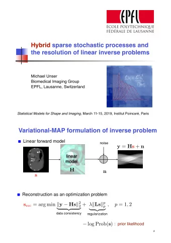
Sparse stochastic processes and biomedical image reconstruction Michael Unser Biomedical Imaging Group EPFL, Lausanne, Switzerland Joint work with P. Tafti, Q. Sun, A. Amini, M. Guerquin-Kern, E. Bostan, etc. Tutorial presentation, FRUMAN, University Aix-Marseille, Feb. 4 2013 . Variational formulation of image reconstruction Linear forward model noise g = Hs + n linear model H n s Ill-posed inverse problem: recover s from noisy measurements g Reconstruction as an optimization problem s ? = argmin ⇥ g � Hs ⇥ 2 + λ R ( s ) 2 | {z } | {z } data consistency regularization 2
Classical linear reconstruction s ? = argmin k g � Hs k 2 + λ R ( s ) 2 | {z } | {z } regularization data consistency Quadratic regularization (Tikhonov) R ( s ) = k Ls k 2 s = ( H T H + λ L T L ) − 1 H T g = R λ · g Formal linear solution: L = C − 1 / 2 m : Whitening filter s Statistical formulation under Gaussian hypothesis Wiener (LMMSE) solution = Gauss MMSE = Gauss MAP 1 σ 2 k g � Hs k 2 k C − 1 / 2 s k 2 s MAP = arg min s + 2 s 2 | {z } | {z } Gaussian prior likelihood Data Log likelihood Signal covariance: C s = E { s · s T } 3 Sparsity-promoting reconstruction algorithms s ? = argmin ⇥ g � Hs ⇥ 2 + λ R ( s ) 2 | {z } | {z } regularization data consistency Wavelet-domain regularization Wavelet expansion: s = Wv (typically, sparse) v = W − 1 s R ( s ) = k v k ` 1 Wavelet-domain sparsity-constraint: with Iterated shrinkage-thresholding algorithm (ISTA, FISTA, FWISTA) ` 1 regularization (Total variation) R ( s ) = k Ls k ` 1 with L : gradient Iterative reweighted least squares (IRLS) or FISTA 4
Key research questions Discretization of reconstruction problem 1 Continuous-domain formulation Generalized sampling Formulation of ill-posed reconstruction problem 2 Statistical modeling (beyond Gaussian) supporting non-linear reconstruction schemes (including CS) Sparse stochastic processes Efficient implementation for large-scale imaging problem 3 FISTA, ADM 5 Lévy processes Constructed by Paul Lévy (circa 1930) 0 0 Gaussian: Brownian motion 0.0 0.2 0.4 0.6 0.8 1.0 Compound Poisson 0 0 0.0 0.2 0.4 0.6 0.8 1.0 S α S (Cauchy) 0 0 0.0 0.2 0.4 0.6 0.8 1.0 Generalization of Brownian motion Independent increments: i.i.d. infinitely divisible (from Gaussian to heavy tailed) Example: compound Poisson process (piecewise-constant with random jumps) ⇒ Archetype of a “sparse” random signal 6
Haar wavelet analysis of a Lévy process Compound Poisson process = piecewise-constant signal Poisson; H = 0.50 D = d s ( x ) d x D ∗ = − d d x (adjoint) D s ( t ) = P n a n δ ( x − x n ) with x n jump locations “Sparse derivative” property: Wavelet as a smoothed derivative ψ Haar ( x ) = D φ ( x ) φ ( x ) ) h s, ψ Haar ( · � y 0 ) i = h s, D φ ( · � y 0 ) i = h D ∗ s, φ ( · � y 0 ) i sparse innovations (train of Dirac impulses) 7 K-term approximation of Lévy processes DCT → Karhunen-Lo` eve transform Sparse: Compound Poisson 8
K-term approximation of Lévy processes DCT → Karhunen-Lo` eve transform Gaussian: Brownian motion 9 K-term approximation of Lévy processes Heavy tailed: Lévy flight (Cauchy) 10
Arguments for continuous-domain formulation ! The real world is continuous ! Input signal ! Imaging physics ! Principled formulation ! Stochastic differential equations (rather than reverse engineering) ! Invariance to coordinate transformations ! Specification of optimal estimators (MAP, MMSE) ! The power of continuous mathematics ! Full backward compatibility with Gaussian theory, link with TV ! Integral operators, characteristic form ! Derivation of joint PDF in any transformed domain (wavelets, gradient, DCT) ! Operational definition of “sparsity” based on existence considerations: infinite divisibility ⇒ processes are either Gaussian or sparse 11 OUTLINE ■ Gaussian (Wiener) vs. sparse (Lévy) signals ✔ ■ The spline connection L -splines and signals with finite rate of innovation ■ Green functions as elementary building blocks ■ ■ Sparse stochastic processes Generalized innovation model ■ Gelfand’s theory of generalized stochastic processes ■ Statistical characterization of sparse stochastic processes ■ ■ Implications of innovation model Link with regularization ■ Wavelet representation of sparse processes ■ Determination of transform-domain statistics ■ ■ Sparse processes and signal reconstruction MAP estimator ■ MRI examples ■ 12
The spline connection Photo courtesy of Carl De Boor 13 Splines: signals with finite rate of innovation L {·} : differential operator δ ( x ) : Dirac distribution Definition The function s ( x ) is a (non-uniform) L -spline with knots { x n } iff. N X L { s } ( x ) = a n δ ( x − x n ) n =1 L = d Spline theory: (Schultz-Varga, 1967) d x a n x n +1 x n FIR signal processing: Innovation variables (2 N ) Location of singularities (knots) : { x n } n =1 ,...,N Strength of singularities (linear weights): { a n } n =1 ,...,N (Vetterli et al., 2002) 14
⇒ Splines and Green’s functions Definition ρ L ( x ) is a Green function of the shift-invariant operator L iff L { ρ L } = δ ρ L ( x ) ρ L ( x ) δ ( x ) L − 1 {·} δ ( x ) L {·} ( + null-space component? ) X General (non-uniform) L -spline: L { s } ( x ) = a k δ ( x − x k ) k ∈ Z Formal integration X L − 1 {·} a k δ ( x − x k ) X s ( x ) = p L ( x ) + a k ρ L ( x − x k ) k ∈ Z k ∈ Z 15 Example of spline synthesis d d x = D ⇒ L − 1 : integrator L = δ ( x ) ρ ( x ) L − 1 {·} Green function = Impulse response Translation invariance δ ( x − x 0 ) ρ ( x − x 0 ) L − 1 {·} Linearity � � a [ k ] δ ( x − k ) s ( x ) = a [ k ] ρ ( x − k ) k ∈ Z k ∈ Z L − 1 {·} 16
Sparse stochastic processes 17 Compound Poisson process (sparse) d ⇒ L − 1 : integrator L = d x X L − 1 {·} s ( x ) r ( x ) = a k δ ( x − x k ) k random stream of Diracs Compound Poisson process 0 0 0.0 0.2 0.4 0.6 0.8 1.0 Random jumps with rate λ (Poisson point process) a v p ( a ) Jump size distribution: (Paul Lévy, 1934) 18
Brownian motion (Gaussian) d ⇒ L − 1 : integrator L = d x Gaussian white noise L − 1 {·} 0 0 0.0 0.2 0.4 0.6 0.8 1.0 Same higher-level properties as Compound Poisson process Non-stationary Except sparsity ! Self-similar: “ 1 / ω ” spectral decay Independent increments = defining property of L´ evy processes Gaussian u [ k ] = s ( k ) − s ( k − 1) : i.i.d. infinitely divisible Cardinal spline (Schoenberg, 1946) 19 Shaping filter L − 1 {·} White noise Generalized (Gaussian, Poisson or Lévy) stochastic process (appropriate boundary conditions) w ( x ) s ( x ) Whitening operator L {·} What is white noise ? The problem : Continuous-domain white noise does not have a pointwise interpretation. Standard stochastic calculus . Statisticians circumvent the difficulty by working with ran- dom measures ( d W ( x ) = w ( x )d x ) and stochastic integrals ; i.e, s ( x ) = R R ρ ( x, x 0 )d W ( x 0 ) where ρ ( x, x 0 ) is a suitable kernel. Innovation model . The white noise interpretation is more appealing for engineers (cf. Papoulis), but it requires a proper distributional formulation and operator calculus.
Road map for theory of sparse processes 2 Specification of inverse operator 3 Characterization of Functional analysis solution of SDE generalized stochastic process Very easy ! (after solving 1. & 2.) L − 1 s = L − 1 w Mixing operator White noise Multi-scale w Whitening operator wavelet L analysis 1 Characterization of continuous-domain white noise 4 Characterization of Higher mathematics: generalized functions (Schwartz) transform-domain statistics measures on topological vector spaces ψ i = L ∗ φ i Easy when: Gelfand’s theory of generalized stochastic processes Infinite divisibility (Lévy-Khintchine formula) 21 Step 1: White noise characterization White noise w s = L − 1 w L − 1 0 5 10 15 20 Whitening operator L Difficulty 1: w 6 = w ( x ) is too rough to have a pointwise interpretation ) X = h w, ϕ i for any ϕ 2 S Difficulty 2: w is an infinite-dimensional random entity; its “pdf” can be formally specified by a measure P w ( E ) where E ⊆ S 0 Infinite-dimensional counterpart of characteristic function (Gelfand, 1955) Z d P w ( ϕ ) = E { e j h w, ϕ i } = S 0 e j h s, ϕ i P w ( ds ) , for any ϕ ∈ S Characteristic functional: White noise property: independence at every point + stationarity 22
Recommend
More recommend
Explore More Topics
Stay informed with curated content and fresh updates.
