Sparse Robust Regression using Non-concave Penalized Density Power - PowerPoint PPT Presentation
Sparse Robust Regression using Non-concave Penalized Density Power Divergence Subhabrata Majumdar Joint work with Abhik Ghosh University of Florida Informatics Institute IISA-2018 conference, Gainesville, FL May 19, 2018 Ghosh and Majumdar
Sparse Robust Regression using Non-concave Penalized Density Power Divergence Subhabrata Majumdar Joint work with Abhik Ghosh University of Florida Informatics Institute IISA-2018 conference, Gainesville, FL May 19, 2018 Ghosh and Majumdar Robust Sparse Regression May 19, 2018
Table of contents Motivation 1 Formulation 2 Influence functions 3 Theory 4 Simulations 5 Ghosh and Majumdar Robust Sparse Regression May 19, 2018
Outline Motivation 1 Formulation 2 Influence functions 3 Theory 4 Simulations 5 Ghosh and Majumdar Robust Sparse Regression May 19, 2018
Penalized linear regression Standard linear regression model (LRM): y = X β + ǫ , where y = ( y 1 , . . . , y n ) T are responses, X = ( x 1 · · · x n ) T is the design matrix, and ǫ = ( ǫ 1 , . . . , ǫ n ) T ∼ N n ( 0 , σ 2 I n ) are the random error components. Ghosh and Majumdar Robust Sparse Regression May 19, 2018
Penalized linear regression Standard linear regression model (LRM): y = X β + ǫ , where y = ( y 1 , . . . , y n ) T are responses, X = ( x 1 · · · x n ) T is the design matrix, and ǫ = ( ǫ 1 , . . . , ǫ n ) T ∼ N n ( 0 , σ 2 I n ) are the random error components. Sparse estimators of β = ( β 1 , . . . , β p ) T , are defined as the minimizer of: n p � � ρ ( y i − x T i β ) + λ n p ( | β j | ) , i = 1 j = 1 where ρ ( . ) is a loss function, p ( . ) is the sparsity inducing penalty function, and λ n ≡ λ is the regularization parameter depending on n . Ghosh and Majumdar Robust Sparse Regression May 19, 2018
Sparse penalized least squares Linear model : y = X β + ǫ , with X ∈ R n × p , β ∈ R p , ǫ ∼ N ( 0 , σ 2 I ) with σ > 0; Lasso (Tibshirani, 1996) n argmin β � y − X β � 2 + λ � β � 1 ; � β = 1 Ghosh and Majumdar Robust Sparse Regression May 19, 2018
Sparse penalized least squares Linear model : y = X β + ǫ , with X ∈ R n × p , β ∈ R p , ǫ ∼ N ( 0 , σ 2 I ) with σ > 0; Lasso (Tibshirani, 1996) n argmin β � y − X β � 2 + λ � β � 1 ; � β = 1 SCAD (Fan and Li, 2001) � β = n � y − X β � 2 + λ � p 1 argmin β j = 1 p ( | β j | ) ; MCP (Zhang, 2010) Ghosh and Majumdar Robust Sparse Regression May 19, 2018
Sparse Robust Regression Sparse versions of robust regression methods- RLARS (Khan et al., 2007), sparse least trimmed squares (Wang et al., 2007), LAD-lasso (Alfons et al., 2013); Robust high-dimensional M-estimation- Neghaban et al. (2012); Bean et al. (2013); Donoho and Montanari (2016); Lozano et al. (2016); Loh and Wainwright (2017) Ghosh and Majumdar Robust Sparse Regression May 19, 2018
Why do we need another? Ghosh and Majumdar Robust Sparse Regression May 19, 2018
Why do we need another? All methods until now focus on ℓ 1 -penalization. But the bias of lasso-type 1 estimators is well-known. Ghosh and Majumdar Robust Sparse Regression May 19, 2018
Why do we need another? All methods until now focus on ℓ 1 -penalization. But the bias of lasso-type 1 estimators is well-known. Many proposed methods lack theoretical rigor and only give algorithms. 2 Ghosh and Majumdar Robust Sparse Regression May 19, 2018
Why do we need another? All methods until now focus on ℓ 1 -penalization. But the bias of lasso-type 1 estimators is well-known. Many proposed methods lack theoretical rigor and only give algorithms. 2 Robustness is either shown empirically or theoretically- not both. 3 Ghosh and Majumdar Robust Sparse Regression May 19, 2018
Why do we need another? All methods until now focus on ℓ 1 -penalization. But the bias of lasso-type 1 estimators is well-known. Many proposed methods lack theoretical rigor and only give algorithms. 2 Robustness is either shown empirically or theoretically- not both. 3 Conditions assumed on the design matrix are largely similar to 4 non-robust cases. Example X T X / n → C (Alfons et al., 2013) Restricted eigenvalue condition (Lozano et al., 2016) Ghosh and Majumdar Robust Sparse Regression May 19, 2018
Outline Motivation 1 Formulation 2 Influence functions 3 Theory 4 Simulations 5 Ghosh and Majumdar Robust Sparse Regression May 19, 2018
The DPD loss function D ensity P ower D ivergence is a generalization of the KL-divergence. DPD-based regression (Durio and Isaia, 2011) maximizes the loss function � � n � 1 − ( 1 + α ) 3 / 2 ( yi − xT i β ) 2 1 1 e − α L α n ( β , σ ) = ( 2 π ) α/ 2 σ α √ 2 σ 2 α n 1 + α i = 1 Ghosh and Majumdar Robust Sparse Regression May 19, 2018
The DPD loss function D ensity P ower D ivergence is a generalization of the KL-divergence. DPD-based regression (Durio and Isaia, 2011) maximizes the loss function � � n � 1 − ( 1 + α ) 3 / 2 ( yi − xT i β ) 2 1 1 e − α L α n ( β , σ ) = ( 2 π ) α/ 2 σ α √ 2 σ 2 α n 1 + α i = 1 Why use DPD? Ghosh and Majumdar Robust Sparse Regression May 19, 2018
The DPD loss function D ensity P ower D ivergence is a generalization of the KL-divergence. DPD-based regression (Durio and Isaia, 2011) maximizes the loss function � � n � 1 − ( 1 + α ) 3 / 2 ( yi − xT i β ) 2 1 1 e − α L α n ( β , σ ) = ( 2 π ) α/ 2 σ α √ 2 σ 2 α n 1 + α i = 1 Why use DPD? Adaptive: Large α = more robust, less efficient. Small α = more robust, less efficient. Ghosh and Majumdar Robust Sparse Regression May 19, 2018
The DPD loss function D ensity P ower D ivergence is a generalization of the KL-divergence. DPD-based regression (Durio and Isaia, 2011) maximizes the loss function � � n � 1 − ( 1 + α ) 3 / 2 ( yi − xT i β ) 2 1 1 e − α L α n ( β , σ ) = ( 2 π ) α/ 2 σ α √ 2 σ 2 α n 1 + α i = 1 Why use DPD? Adaptive: Large α = more robust, less efficient. Small α = more robust, less efficient. Generalized: As α ↓ 0, L α n ( β , σ ) coincides (in a limiting sense) with the negative log-likelihood. (why? think L-Hospital’s rule.) Ghosh and Majumdar Robust Sparse Regression May 19, 2018
Penalized DPD p � L α n ( β , σ ) + p λ ( | β j | ) j = 1 where p λ ( · ) is a penalty function (lasso, SCAD, MCP , ...). Ghosh and Majumdar Robust Sparse Regression May 19, 2018
Penalized DPD p � L α n ( β , σ ) + p λ ( | β j | ) j = 1 where p λ ( · ) is a penalty function (lasso, SCAD, MCP , ...). As α ↓ 0, this becomes the (non-robust) non-concave penalized negative log-likelihood. Ghosh and Majumdar Robust Sparse Regression May 19, 2018
Computational algorithm Starting from ˆ β , ˆ σ , Iteratively minimize the following: p � R α λ ( β ) = L α n ( β , ˆ σ ) + p λ ( | β j | ) , j = 1 S α ( σ ) = L α n (ˆ β , σ ) . Ghosh and Majumdar Robust Sparse Regression May 19, 2018
Computational algorithm Starting from ˆ β , ˆ σ , Iteratively minimize the following: p � R α λ ( β ) = L α n ( β , ˆ σ ) + p λ ( | β j | ) , j = 1 S α ( σ ) = L α n (ˆ β , σ ) . Update β using a Concave-Convex Procedure (CCCP): p λ ( | β j | ) = ˜ J λ ( | β j | ) + λ | β j | ≃ ∇ ˜ J λ ( | β c j | ) β j + λ | β j | J ( · ) is differentiable and concave, β c is a current solution. where ˜ Update σ using gradient descent. Ghosh and Majumdar Robust Sparse Regression May 19, 2018
Updating ˆ β and ˆ σ Ghosh and Majumdar Robust Sparse Regression May 19, 2018
Updating ˆ β and ˆ σ � σ ( k ) � p � � � ( k + 1 ) = argmin ∇ ˜ β ( k ) ˆ L α J λ ( | ˆ β β , ˆ + | ) β j + λ | β j | ; n j β j = 1 Ghosh and Majumdar Robust Sparse Regression May 19, 2018
Updating ˆ β and ˆ σ � σ ( k ) � p � � � ( k + 1 ) = argmin ∇ ˜ β ( k ) ˆ L α J λ ( | ˆ β β , ˆ + | ) β j + λ | β j | ; n j β j = 1 � n � � n � − 1 � i β ( k + 1 ) � 2 � � α σ 2 ( k + 1 ) = w ( k ) w ( k ) y i − x T ˆ − , i i ( 1 + α ) 3 / 2 i = 1 i = 1 � � i β ( k ) ) 2 − α ( y i − x T w ( k ) := exp . i σ 2 ( k ) Ghosh and Majumdar Robust Sparse Regression May 19, 2018
Tuning parameter selection To choose λ , we use a robust High-dimensional BIC: σ 2 ) + log log( n ) log p � ˆ HBIC ( λ ) = log(ˆ β � 0 , (1) n and select the optimal λ ∗ that minimizes the HBIC over a pre-determined set of values Λ n : λ ∗ = argmin λ ∈ Λ n HBIC ( λ ) . Ghosh and Majumdar Robust Sparse Regression May 19, 2018
Outline Motivation 1 Formulation 2 Influence functions 3 Theory 4 Simulations 5 Ghosh and Majumdar Robust Sparse Regression May 19, 2018
Definition The Influence Function (IF) is a classical tool of measuring the asymptotic local robustness of any estimator (Hampel, 1968, 1974). Ghosh and Majumdar Robust Sparse Regression May 19, 2018
Recommend
More recommend
Explore More Topics
Stay informed with curated content and fresh updates.
