Sparse Canonical Correlation Analysis: Minimaxity, Algorithm, and - PowerPoint PPT Presentation

Sparse Canonical Correlation Analysis: Minimaxity, Algorithm, and Computational Barrier Harrison H. Zhou Department of Statistics Yale University 1

Chao Gao Mengjie Chen Zongming Ma Zhao Ren 2

Outline • Introduction to Sparse CCA • An Elementary Reparametrization of CCA • A Naive Methodology and Its Theoretical Justification • Minimaxity, Algorithm, and Computational Barrier 3

Introduction to Sparse CCA 4

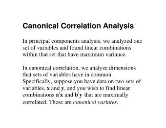
What Is CCA? Find θ and η : max Cov( θ T X, η T Y ) , s.t. Var( θ T X ) = Var( η T Y ) = 1 , where      Σ x Σ xy  X  =  . Cov Σ yx Σ y Y (Hotelling 1936) 5

Oracle Solution Find θ and η : max θ T Σ xy η, s.t. θ T Σ x θ = η T Σ y η = 1 . Solution : Σ 1 / 2 x θ and Σ 1 / 2 y η are the first singular pair of Σ − 1 / 2 Σ xy Σ − 1 / 2 . x y 6

Sample Version Find θ and η : max θ T ˆ s.t. θ T ˆ Σ x θ = η T ˆ Σ xy η, Σ y η = 1 . Solution : ˆ x θ and ˆ y η are the first singular pair of ˆ Σ xy ˆ ˆ Σ 1 / 2 Σ 1 / 2 Σ − 1 / 2 Σ − 1 / 2 . x y Concerns: Let X ∈ R p and Y ∈ R m . When p ∧ m ≫ n , • Estimation may not be consistent. • The performance of ˆ Σ − 1 / 2 and ˆ Σ − 1 / 2 can be poor. x y 7

Sparse CCA Impose sparsity on θ and η . 8

An Attempt to Sparse CCA PMD (Penalized Matrix Decomposition) Witten, Tibshirani & Hastie (2009) Find θ and η : max θ T ˆ s.t. θ T θ ≤ 1 , η T η ≤ 1 , Σ xy η, || θ || 1 ≤ c 1 , || η || 1 ≤ c 2 . Main Ideas: • Impose sparsity. • “Estimate” Σ x and Σ y by identity matrices. 9

An Attempt to Sparse CCA - Cont. Some concerns: • Computation: the problem is not convex (bi-convex). • Theory: no theoretical guarantee for the global maximizer. • Bias: consequence of using identities is unclear. 10

Simulation result when Σ x and Σ y are not identities (n=500) Truth 0.20 0.00 0 100 200 300 400 CAPIT 0.4 0.2 0.0 0 100 200 300 400 PMD 0.0 −0.6 0 100 200 300 400 11

An Elementary Reparametrization of CCA 12

Reparametrization Find θ and η : max θ T Σ xy η, s.t. θ T Σ x θ = η T Σ y η = 1 . Reparametrization : Σ xy = Σ x A Σ y . SVD w.r.t. Σ x and Σ y : A = ΘΛ H T , Θ T Σ x Θ = H T Σ y H = I, for some Θ = [ θ 1 , θ 2 , ..., θ r ] , H = [ η 1 , η 2 , ..., η r ], and Λ = diag( λ 1 , ..., λ r ) with λ i deceasing. 13

An Explicit Solution Find θ and η : max θ T Σ xy η, s.t. θ T Σ x θ = η T Σ y η = 1 . Solution : θ = σθ 1 , η = ση 1 , where σ = ± 1. 14

The Single Canonical Pair (SCP) Model Let r = 1, we have Σ xy = λ Σ x θη T Σ y , θ T Σ x θ = η T Σ y η = 1 . Sparse CCA for r = 1 : • The rank one matrix Ω x Σ xy Ω y has a sparse decomposition λθη T , where Ω x = Σ − 1 x , and Ω y = Σ − 1 y • We assume the vectors θ and η have at most s non-zero coordinates. 15

Comparison: The Single Spike Model (Johnstone & Lu, 2009) Σ = λθθ T + I, θ T θ = 1 . • Sparse CCA is harder: extra nuisance parameters Σ x and Σ y . • Sparsity of θ, η may not imply sparsity of Σ xy . 16

A Naive Methodology and Its Theoretical Justification 17

Known Covariance Observations : { ( X i , Y i ) } n i =1 i.i.d.     λ Σ x θη T Σ y Σ x  X i  =   . Cov λ Σ y ηθ T Σ x Σ y Y i Transformation :     λθη T  Ω x X i  Ω x  =  . Cov ληθ T Ω y Y i Ω y Unbiased estimator of A = λθη : ∑ n A = 1 ˆ Ω x X i Y T i Ω y . n i =1 Apply sparse SVD to ˆ A . 18

CCA via Precision adjusted Iterative Thresholding Step 1: Splitting the data into two halves. Use the first half data to form Ω x , ˆ ˆ Ω y . Step 2: Apply coordinate thresholding on the matrix n ∑ A = 2 ˆ ˆ i ˆ Ω x X i Y T Ω y . n i = n/ 2+1 to get an initializer u (0) or v (0) . A with the initializer and get u ( k ) and Step 3: Apply iterative thresholding on ˆ v ( k ) . 19

Convergence Rate of CAPIT - Assumptions Assumption A:  ) 1 / 2  ( n   . s = o log p Assumption B: || (ˆ Ω x Σ x − I ) θ || ∨ || (ˆ Ω y Σ y − I ) η || = o P (1) . In addition, we assume that λ ≥ M − 1 , || Σ x || ∨ || Σ y || ∨ || Ω x || ∨ || Ω y || ≤ M. 20

Convergence Rate of CAPIT - Loss Function Consider the joint loss L 2 (ˆ θ, θ ) + L 2 (ˆ η, η ) θ, θ ) | 2 + | sin ∠ (ˆ | sin ∠ (ˆ η, η ) | 2 . = 21

Convergence Rate of CAPIT Theorem 1 Under the assumptions, we have, s log p L 2 (ˆ θ, θ ) + L 2 (ˆ η, η ) ≲ n Ω x Σ x − I ) θ || 2 + || (ˆ || (ˆ Ω y Σ y − I ) η || 2 , + with high probability. 22

Remark The convergence rate depends on || (ˆ Ω x Σ x − I ) θ || + || (ˆ Ω y Σ y − I ) η || , determined by the covariance class F p . Example of F p : Bandable, Sparse, Toeplitz, Graphical Model, Spiked Covariance... 23

Minimaxity 24

Questions on Fundamental Limits • Go beyond r = 1? • Allow to have residual canonical correlation directions? • Avoid the ugly terms in Theorem 1? 25

General Sparse CCA Model: ( ) U 1 Λ 1 V T 1 + U 2 Λ 2 V T U T Σ x U = V T Σ y V = I, Σ xy = Σ x Σ y , 2 where U = [ U 1 , U 2 ] , V = [ V 1 , V 2 ] . Goal: estimating sparse U 1 and V 1 (at most s nonzero rows). No structural assumption on U 2 , V 2 , Σ x , Σ y . 26

Procedure The estimator ( � U 1 , � V 1 ) is a solution to the following optimization problem, tr ( A ′ � max Σ xy B ) ( A,B ) s.t. A ′ � Σ x A = B ′ � Σ y B = I r and exactly s nonzero rows for both A and B, where � Σ x , � Σ y , and � Σ xy are sample covariance matrices. 27

Assumptions • U 1 ∈ R p × r and V 1 ∈ R m × r have at most s number of nonzero rows; • 1 > κλ ≥ λ 1 ≥ ... ≥ λ r ≥ λ > 0; • λ r +1 ≤ cλ r for some c small; � � � � � Σ l � � Σ l � • op ∨ op ≤ M for l = ± 1. x y 28

Minimaxity Theorem 2 Under the assumptions, we have, 1 − � E || U 1 V ′ 1 || 2 U 1 V ′ inf sup F � Σ ∈F 0 ( s,p,m,r,λ ) U 1 V ′ 1 1 nλ 2 [ rs + s (log p s + log m ≍ s )] . 29

Remarks: • We allow arbitrary r as results for sparse PCA. • The presence of the residual canonical correlation directions do not influence the minimax rates under a mild condition on eigengap. • The minimax rates are not affected by estimation of Σ − 1 and Σ − 1 y . x 30

Algorithm 31

Questions on Computational Feasibility A polynomial time algorithm to • Go beyond r = 1? • Allow to have residual canonical correlation directions? • Avoid the ugly terms? Answer : Not yet. We need to assume residual canonical correlation directions to be zero, i.e., U 2 = 0 or V 2 = 0. 32

Two-Stage Procedure: I Initialization by Convex Programming tr ( � Σ xy F ′ ) − ρ || F || 1 , maximize || � x F � Σ 1 / 2 Σ 1 / 2 subject to y || ∗ ≤ r, || � x F � Σ 1 / 2 Σ 1 / 2 y || spectral ≤ 1 . Motivation: Exhaustive search procedure tr ( A ′ � max Σ xy B ) ( A,B ) s.t. A ′ � Σ x A = B ′ � Σ y B = I r and exactly s nonzero rows for both A and B. 33

Two-Stage Procedure: II Refinement by Sparse Regression – Group Lasso { } p ∑ � tr ( L ′ � Σ x L ) − 2 tr ( L ′ � Σ xy V (0) ) + ρ u U = arg min || L j · || , L ∈ R p × r j =1 { } m ∑ � tr ( R ′ � Σ y R ) − 2 tr ( R ′ � Σ yx U (0) ) + ρ v V = arg min || R j · || . R ∈ R m × r j =1 Motivation: Least square solutions L ∈ R p × r E || L ′ X − V ′ Y || 2 R ∈ R m × r E || R ′ Y − U ′ X || 2 min min F , F . The minimizers are U Λ and V Λ. 34

Statistical Optimality Assume that s 2 log( p + m ) ≤ c, nλ 2 r for some sufficiently small c ∈ (0 , 1). We can show that C s ( r + log p ) U − P U || 2 || P � ≤ , F nλ 2 r C s ( r + log m ) V − P V || 2 || P � ≤ , F nλ 2 r with high probability. 35

Computational Barrier 36

Computational Barrier Consider r = 1. There is a set of Gaussian distributions G such that for some δ ∈ (0 , 1) with s 2 − δ log( p + m ) lim > 0 , nλ 2 n →∞ then for any randomized polynomial-time estimator ˆ U , U − P U || 2 n →∞ sup lim E || P � F > c, G for some constant c > 0 under the assumption that the Planted Clique Hypothesis holds. 37

Summary • An elementary characterization of Sparse CCA is provided. • A preliminary adaptive procedure (CAPIT) is proposed, but needs to take advantage of the covariance structure. • Minimax rate for Sparse CCA is nailed down, but the upper bound is achieved through exhaustively searching the support. • A new computationally feasible algorithm attains the minimax rate, but need to assume residual canonical correlation directions to be zero. • A computational barrier. 38