Canonical Correlation a Tutorial Magnus Borga January 12, 2001 - PDF document

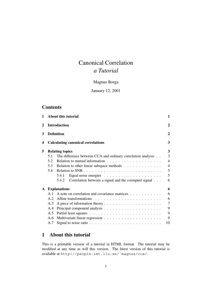
Canonical Correlation a Tutorial Magnus Borga January 12, 2001 Contents 1 About this tutorial 1 2 Introduction 2 3 Definition 2 4 Calculating canonical correlations 3 5 Relating topics 3 5.1 The difference between CCA and ordinary correlation analysis . . 3 5.2 Relation to mutual information . . . . . . . . . . . . . . . . . . . 4 5.3 Relation to other linear subspace methods . . . . . . . . . . . . . 4 5.4 Relation to SNR . . . . . . . . . . . . . . . . . . . . . . . . . . . 5 5.4.1 Equal noise energies . . . . . . . . . . . . . . . . . . . . 5 5.4.2 Correlation between a signal and the corrupted signal . . . 6 A Explanations 6 A.1 A note on correlation and covariance matrices . . . . . . . . . . . 6 A.2 Affine transformations . . . . . . . . . . . . . . . . . . . . . . . 6 A.3 A piece of information theory . . . . . . . . . . . . . . . . . . . . 7 A.4 Principal component analysis . . . . . . . . . . . . . . . . . . . . 9 A.5 Partial least squares . . . . . . . . . . . . . . . . . . . . . . . . . 9 A.6 Multivariate linear regression . . . . . . . . . . . . . . . . . . . . 9 A.7 Signal to noise ratio . . . . . . . . . . . . . . . . . . . . . . . . . 10 1 About this tutorial This is a printable version of a tutorial in HTML format. The tutorial may be modified at any time as will this version. The latest version of this tutorial is available at http://people.imt.liu.se/˜magnus/cca/ . 1

2 Introduction Canonical correlation analysis (CCA) is a way of measuring the linear relationship between two multidimensional variables. It finds two bases, one for each variable, that are optimal with respect to correlations and, at the same time, it finds the corresponding correlations. In other words, it finds the two bases in which the correlation matrix between the variables is diagonal and the correlations on the diagonal are maximized. The dimensionality of these new bases is equal to or less than the smallest dimensionality of the two variables. An important property of canonical correlations is that they are invariant with respect to affine transformations of the variables. This is the most important differ- ence between CCA and ordinary correlation analysis which highly depend on the basis in which the variables are described. CCA was developed by H. Hotelling [10]. Although being a standard tool in statistical analysis, where canonical correlation has been used for example in economics, medical studies, meteorology and even in classification of malt whisky, it is surprisingly unknown in the fields of learning and signal processing. Some exceptions are [2, 13, 5, 4, 14], For further details and applications in signal processing, see my PhD thesis [3] and other publications. 3 Definition Canonical correlation analysis can be defined as the problem of finding two sets of basis vectors, one for x and the other for y , such that the correlations between the projections of the variables onto these basis vectors are mutually maximized. Let us look at the case where only one pair of basis vectors are sought, namely the ones corresponding to the largest canonical correlation: Consider the linear T T x = x w ^ y = y w ^ combinations x and y of the two variables respectively. This means that the function to be maximized is T T [ xy ℄ [ ℄ E E w ^ xy w ^ y x � = = p q E [ x 2 ℄ E [ y 2 ℄ T T T T E [ w ^ xx w ^ ℄ E [ w ^ yy w ^ ℄ x y x y (1) T w C w xy y x = : q T T w C w w C w xx x y y y x y The maximum of � with respect to w x and w y is the maximum canonical correlation. The subsequent canonical correlations are uncorrelated for different solutions, i.e. 8 T T T E [ x x ℄ = E [ w xx w ℄ = w C w = 0 i j xj xx xj xi xi > < T T T [ y ℄ = [ w ℄ = = 0 for i 6 = j: (2) E y E yy w w C w i j y j y y y j y i y i > T T T [ x ℄ = [ w ℄ = = 0 E y E xy w w C w : i j y j xy y j xi xi 2

The projections onto w x and w y , i.e. x and y , are called canonical variates . 4 Calculating canonical correlations Consider two random variables x and y with zero mean. The total covariance matrix " T # � � � � � � C C x x xx xy = = E C (3) C C y y y x y y is a block matrix where C xx and C xx are the within-sets covariance matrices of x T = and y respectively and C C x is the between-sets covariance matrix. xy y The canonical correlations between x and y can be found by solving the eigen- value equations ( � 1 � 1 2 = � C C C C w ^ w ^ xy y x x x xx y y (4) � 1 � 1 2 = C C C C w ^ � w ^ y x xy y y y y xx 2 are the squared canonical correlations and the eigen- where the eigenvalues � vectors w ^ x and w ^ y are the normalized canonical correlation basis vectors . The number of non-zero solutions to these equations are limited to the smallest dimen- sionality of x and y . E.g. if the dimensionality of x and y is 8 and 5 respectively, the maximum number of canonical correlations is 5. Only one of the eigenvalue equations needs to be solved since the solutions are related by 8 = C w ^ �� C w ^ xy y x xx x < (5) = C w ^ �� C w ^ ; : y x x y y y y where s T w ^ C w ^ y y y y � 1 � = � = : (6) x y T w ^ C w ^ xx x x 5 Relating topics 5.1 The difference between CCA and ordinary correlation analysis Ordinary correlation analysis is dependent on the coordinate system in which the variables are described. This means that even if there is a very strong linear rela- tionship between two multidimensional signals, this relationship may not be visible in a ordinary correlation analysis if one coordinate system is used, while in another coordinate system this linear relationship would give a very high correlation. CCA finds the coordinate system that is optimal for correlation analysis, and the eigenvectors of equation 4 defines this coordinate system. 3

Example: Consider two normally distributed two-dimensional variables x and y with unit variance. Let y + y = x + x 2 . It is easy to confirm that the correlation 1 2 1 matrix between x and y is � � 0 : 5 0 : 5 = : R (7) xy 0 : 5 0 : 5 This indicates a relatively weak correlation of 0.5 despite the fact that there is a perfect linear relationship (in one dimension) between x and y . A CCA on this data shows that the largest (and only) canonical correlation is T in which this perfect linear relationship one and it also gives the direction [11℄ lies. If the variables are described in the bases given by the canonical correlation basis vectors (i.e. the eigenvectors of equation 4), the correlation matrix between the variables is � � 1 0 R = : (8) xy 0 1 5.2 Relation to mutual information There is a relation between correlation and mutual information. Since informa- tion is additive for statistically independent variables and the canonical variates are uncorrelated, the mutual information between x and y is the sum of mutual x y information between the variates i and i if there are no higher order statistic de- pendencies than correlation (second-order statistics). For Gaussian variables this means 1 � 1 � 1 � 1 � X ( x ; ) = log = log I y : (9) 2 2 2 Q (1 � ) 2 (1 � ) � � i i i i Kay [13] has shown that this relation plus a constant holds for all elliptically sym- metrical distributions of the form T � 1 (( z � � ) ( z � � z )) : f z C (10) 5.3 Relation to other linear subspace methods Instead of the two eigenvalue equations in 4 we can formulate the problem in one single eigenvalue equation: � 1 B A w ^ = � w ^ (11) where � � � � � � 0 C C 0 � w ^ xy xx x x = ; = = : A B and w ^ (12) C 0 0 C � w ^ y x y y y y Solving the eigenproblem in equation 11 with slightly different matrices will give solutions to principal component analysis (PCA), partial least squares (PLS) and multivariate linear regression (MLR). The matrices are listed in table 1. 4

A B C I PCA xx � � � � 0 C I 0 xy PLS C 0 0 I y x � � � � 0 C C 0 xy xx CCA C 0 0 C y x y y � � � � 0 C C 0 xy xx MLR C 0 0 I y x Table 1: The matrices A and B for PCA, PLS, CCA and MLR. 5.4 Relation to SNR Correlation is strongly related to signal to noise ratio (SNR), which is a more com- x and two noise signals monly used measure in signal processing. Consider a signal 2 all having zero mean 1 and all being uncorrelated with each other. Let � 1 and � 2 2 S = E [ x ℄ and N = E [ � ℄ be the energy of the signal and the noise signals i i respectively. Then the correlation between a ( x + � ) and b ( x + � ) is 1 2 E [ a ( x + � ) b ( x + � )℄ 1 2 � = p E [ a 2 ( x + � ) 2 ℄ E [ b 2 ( x + � ) 2 ℄ 1 2 � � 2 E x = (13) q � � 2 �� � � 2 �� E [ x 2 ℄ + E � E [ x 2 ℄ + E � 1 2 S = : p ( S + )( S + ) N N 1 2 Note that the amplification factors a and b do not affect the correlation or the SNR. 5.4.1 Equal noise energies In the special case where the noise energies are equal, i.e. N = N = N , equation 13 can be written as 1 2 S � = : (14) S + N This means that the SNR can be written as S � = : (15) N 1 � � 1 The assumption of zero mean is for convenience. A non-zero mean does not affect the SNR or the correlation. 5