Canonical Correlation Analysis In principal components analysis, we - PowerPoint PPT Presentation
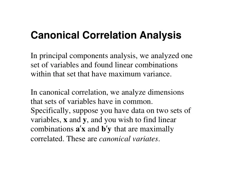
Canonical Correlation Analysis In principal components analysis, we analyzed one set of variables and found linear combinations within that set that have maximum variance. In canonical correlation, we analyze dimensions that sets of variables
Canonical Correlation Analysis In principal components analysis, we analyzed one set of variables and found linear combinations within that set that have maximum variance. In canonical correlation, we analyze dimensions that sets of variables have in common. Specifically, suppose you have data on two sets of variables, x and y , and you wish to find linear combinations ′ a x and ′ b y that are maximally correlated. These are canonical variates .
Another view of Canonical Variates An alternate view of the first canonical variate in one set of variables is that it is the linear combination of those variables that has the highest multiple correlation with the variables in the other set.
What Are They Used For Example. The relationship between personality and achievement is of interest. Suppose the x variables are a set of personality scale scores, and the y variables are a set of academic achievement scores. Then the first canonical variate may isolate dimensions of personality and achievement that predict each other well.
Finding the Canonical Variates Finding the canonical variates amounts to finding the linear weights a and b that generate them. These linear weights can of course only be identified by shape. Multiplying a or b by a constant will not change the correlation between ′ ′ = a x and v = b y . the canonical variates u
So we implement the unit variance restrictions ′ ′ = = a S a b S b 1 (1) i xx i i yy i A straightforward application of matrix calculus leads to the result that the a corresponding to the i i th canonical variate is proportional to the eigenvectors of the quadruple product − − 1 1 S S S S (2) xx xy yy yx 2 and that the squared canonical correlation r is the i corresponding eigenvalue. The canonical weights
for the y variates are obtained from the eigenvectors of − − 1 1 S S S S (3) yy yx xx xy It is important to realize that textbooks, in general, are very confused (or at least very confusing) in their treatments of canonical correlation. In particular, there are different meanings of the same term, depending on which book you read.
Raw Canonical Coefficients (Weights) These are the linear weights used to produce the canonical variates from the raw scores. Note, however, our previous restriction that the canonical variates have unit variance as per Equation (1). Since the eigenvectors as output from most computer software are normalized to have “unit length”, i.e., ′ = a a 1 (4) i i
they will not generally satisfy Equation (1). What to do? In essence, we find out the variance of the variable created from the normalized eigenvectors, then restandardize each vector to produce a variance of 1. In a while, we will see how this is done using a symmetric power of a matrix. This creates a paradox. Suppose that a variable in the y set is perfectly reproduced from a linear combination of the variables in the x set, but that the variable in the y set does not have unit variance. Then the “raw canonical weights” after they are corrected will not produce a variable equal
to the variable in the y set. It will be perfectly correlated with it. On the other hand, the canonical weights before being corrected will produce scores identical to the variable in the y set. So there are, in fact, 3 versions of canonical coefficients we may talk about. 1. Completely raw. Based on the eigenvectors in Equations (2) and (3). 2. Partially standardized . Rescaled so that the canonical variates computed from raw scores in x and y have unit variance.
3. Completely standardized . Based on standardized x and y (i.e., calculated from correlation matrices rather than covariance matrices), then rescaled so that the canonical variates computed from the standardized scores have unit variance. Let’s use score notation. The “partially standardized” canonical variates for the x set are produced as − ′ = = 1/ 2 * U XA A S A ( ) XA (5) xx and those for the y set are
− ′ = = 1/ 2 * V YB B S B ( ) YB (6) yy where A has in its columns the eigenvectors of the matrix in Equation (2), and B has the eigenvectors * * A and B are in of the matrix in Equation (3). actually the “raw canonical weights” referred to by the SAS program. If correlation matrices rather than covariance matrices are used in Equations (2) and (3), then the * * A and B are the completely resulting standardized weights referred to as “standardized canonical weights” by the SAS program.
Recommend
More recommend
Explore More Topics
Stay informed with curated content and fresh updates.

