Sound Processing and Digital Filters Graduate School of Culture - PowerPoint PPT Presentation
CTP 431 Music and Audio Computing Sound Processing and Digital Filters Graduate School of Culture Technology (GSCT) Juhan Nam 1 Outlines Introduction: Sound Processing Linear Time-Invariant Digital Filter Impulse response
CTP 431 Music and Audio Computing Sound Processing and Digital Filters Graduate School of Culture Technology (GSCT) Juhan Nam 1
Outlines § Introduction: Sound Processing § Linear Time-Invariant Digital Filter – Impulse response – Convolution § Digital Filters – FIR Filters – IIR Filters § Frequency Response § Transfer functions – Z-transform – Pole-Zero Analysis § Bi-quad Filters 2
Introduction: Sound Processing § Sounds captured on computers are processed in various ways – Sample editing: cut, copy, paste – Amplitude: gain, fade in/out, automation curve, compressor – Timbre: lowpass/highpass filters, EQ, distortion, modulation – Spatial effect: delay, reverberation – Pitch: pitch shifting (e.g. auto-tune) – Time stretching – Noise suppression 3
Sound Processing Input Processor Output § Linear processing – No sinusoidal components are introduced by the processing • Only the amplitude and phase of sinusoidal components of the input change – Filters (lowpass, highpass, bandpass, …), EQ – Delay-based audio effect: delay, chorus, flanger, reverberation § Non-linear processing – New sinusoidal components are generated – Compressor, distortion, clipping – Pitch shifting, ring modulation, … 4
Linear Time-Invariant (LTI) Digital Filters Output Input Filter x ( n ) y ( n ) § What linear filters can do – Amplifying the input (or the past output): e.g. y ( n ) = a x ( n ) – Delaying the input (or the past output): e.g. y ( n ) = x ( n-1 ) – Summing them all: y ( n ) = a x ( n ) + x ( n-1 ) § “Easy-to-understand” definition 5
LTI Digital Filters (Formal) Output Input Filter x ( n ) y ( n ) § Linearity – Homogeneity: if x(n) à y(n) , a x(n) à a y(n) – Superposition: if x 1 (n) à y 1 (n) and x 2 (n) à y 2 (n), x 1 (n) + x 2 (n) à y 1 (n) + y 2 (n) § Time-Invariance – If x(n) à y(n) , x(n-N) à y(n-N) for any N – The system does not change its behavior with time. • In practice, most systems do change over time but not quickly 6
Example: Simple LTI Digital Filters § Moving-average filter – y ( n ) = 0.5 x ( n ) + 0.5 x ( n -1) – Low-pass § Differentiator – y ( n ) = 0.5 x ( n ) - 0.5 x ( n -1) – High-pass § Feed-forward comb filter – y ( n ) = x ( n ) + x ( n -M) where M is, say,100 – Renders harmonically distributed peaks and valleys 7
Impulse Response Output Input Filter x(n) = δ (n) h ( n ) y(n) = h(n) § Characterize filters as a number sequence § Obtained when x(n) is a unit impulse – x(n) = δ (n) = [1, 0, 0, 0, …] à y(n) = h(n) § Can be measured from a linear system (black-box approach) – If you excite the linear system with an impulse, you can record the output and use that to determine exactly what the system response would be to any arbitrary input. 8
Convolution § The output of LTI systems is represented by convolution operation between the input x(n) and impulse response h(n) M ∑ y ( n ) = x ( n )* h ( n ) = x ( i ) h ( n − i ) i = 0 § Deriving convolution – The input is decomposed into a time-ordered set of weighted impulse • x(n) = [ x 0, x 1, x 2, x 3, … , x M, ] � = x 0 δ (n) + x 1 δ (n-1) + x 2 δ (n-2) + x 3 δ (n-3) + …+ x M δ (n-M) – By the linearity and time-invariance • y(n) = x 0 h(n) + x 1 h(n-1) + x 2 h(n-2) + x 3 h(n-3) + …+ x M h(n-M) 9
Convolution in Practice § From the commutative law M M ∑ ∑ y ( n ) = x ( n )* h ( n ) = x ( i ) h ( n − i ) x ( n − i ) h ( i ) = i = 0 i = 0 – y(n) = h 0 x(n) + h 1 x(n-1) + h 2 x(n-2) + h 3 x(n-3) + …+ h M x(n-M) – For example: x(n) (n=0,1,2,3,4,5) , h(n) = [ h 0 h 1 h 2 ] • y(0) = h 0 x(0) Transient region • y(1) = h 0 x(1) + h 1 x(0) • y(2) = h 0 x(2) + h 1 x(1) + h 2 x(0) • y(3) = h 0 x(3) + h 1 x(2) + h 2 x (1) Fully overlapped region • y(4) = h 0 x(4) + h 1 x(3) + h 2 x (2) (steady-state) • y(5) = h 0 x(5) + h 1 x(4) + h 2 x (3) • y(6) = h 1 x(5) + h 2 x (4) Transient region • y(7) = h 2 x (5) 10
Convolution in Practice § If the length of x(n) is M and the length of h(n) is N , the length of y(n) is M+N-1 § Computation Complexity – In Big-O notation, it requires M x N multiplications – If N is a large number, it is quite expensive to compute – We can compute convolution in frequency domain, which is much cheaper than the time-domain approach when the impulse response is long (e.g. reverberation or head-related transfer functions) 11
Properties of LTI systems § Commutative x ( n )* h 1 ( n )* h 2 ( n ) = x ( n )* h 2 ( n )* h 1 ( n ) § Associative { x ( n )* h 1 ( n )}* h 2 ( n ) = x ( n )*{ h 1 ( n )* h 2 ( n )} § Distributive x ( n )* h 1 ( n ) + x ( n )* h 2 ( n ) = x ( n )*{ h 1 ( n ) + h 2 ( n )} 12
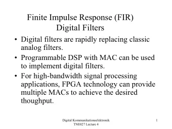
FIR Filters § The output is formed from input and its past input – They have finite impulse responses (FIR) – Convolution with the finite impulse responses y ( n ) = b 0 x ( n ) + b 1 x ( n − 1) + b 2 x ( n − 2) + ... + b M x ( n − M ) x(n) y(n) + b 0 Z -1 x(n-1) b 1 Z -1 Z -1 x(n-2) . . “Delay operator” . b 2 (a unit sample of delay) Z -1 x(n-M) b M 13
IIR Filters § The output can be also formed by input and past outputs – The feedback creates an infinite impulse response! – Convolution with the infinite impulse responses y ( n ) = b 0 x ( n ) − a 1 y ( n − 1) − a 2 y ( n − 2) − ... − b N y ( n − N ) x(n) + y(n) b 0 Z -1 y(n-1) -a 1 Z -1 y(n-2) . . . -a 2 Z -1 y(n-M) -a N 14
IIR Filters § The infinite impulse response – For example: y ( n ) = x ( n ) + ry ( n-1 ) • y (0) = x (0) • y (1) = x (1) + ry (0) = x (1) + rx (0) • y (2) = x (2) + ry (1) = x (2) + rx (1) + r 2 x (0) • y (3) = x (3) + ry (2) = x (3) + rx (2) + r 2 x (1) + r 3 x (0) • y (4) = x (4) + ry (3) = x (4) + rx (3) + r 2 x (2) + r 3 x (1) + r 4 x (0) à h ( n ) = [1 r r 2 r 3 r 4 r 5 r 6 …] – Stability issue! • If r < 1, the filter becomes stable • If r =1, the filter oscillates • If r > 1, the filter becomes unstable – The impulse response is long but, in practice, it is finite (for r < 1) because the level goes below the the quantization noise floor 15
Example: IIR Filters § Leaky Integrator – y ( n ) = x ( n ) + ry ( n-1 ) – r is a slightly less than 1. (1-r) is the “leak” – Lowpass filtering § “Reson” filter – y ( n ) = x ( n ) +2rcos θ y ( n-1 ) - r 2 y ( n-2 ) – r controls the resonance and θ controls its frequency • Resonance: 0 (low resonance) < r < 1 (low resonance) • Cut-off frequency (f c ): θ =2 π f c /f s (f s : sampling rate) – Low-pass/band-pass/high-pass filtering depending on additional zeros § Feed-back comb filter – y ( n ) = x ( n ) + ry ( n -M) – Renders a harmonic tone 16
General Filter Form § The general form of digital Filters y ( n ) = b 0 x ( n ) + b 1 x ( n − 1) + b 2 x ( n − 2) + ... + b M x ( n − M ) “Difference EquaLon” − a 1 y ( n − 1) − a 2 y ( n − 2) − ... − a N y ( n − N ) – The order of the filter is the greater of M or N y(n) x(n) + b 0 Z -1 Z -1 x(n-1) y(n-1) -a 1 b 1 Z -1 Z -1 x(n-2) y(n-2) . . . . . . b 2 -a 2 Z -1 Z -1 y(n-N) x(n-M) -a N b M 17
Filter Implementation Forms § Direct Form I y(n) + x(n) b 0 Z -1 Z -1 -a 1 b 1 Z -1 Z -1 -a 2 b 2 ( By the commutative rule) § Direct Form II y(n) x(n) + + b 0 Z -1 -a 1 b 1 “Biquad Filter” Z -1 -a 2 b 2 18
Example of Filter Implementation § Typically implemented in time-domain A short version using “filter” function in Matlab 19
Frequency Responses § Describe the characteristics of filters in frequency domain – Amplitude response: the amount of amplitude change (often in dB) – Phase response: the amount of delay (-2pi ~ 0) Amplitude Response Phase Response 30 0 − 0.5 20 − 1 10 Gain(dB) radian − 1.5 0 − 2 − 10 − 2.5 − 20 − 3 − 30 2 3 4 2 3 4 10 10 10 10 10 10 freqeuncy(log10) freqeuncy(log10) 20
Frequency Responses Input Output Filter x(n) = e j ω n y(n) = G ( ω )e j( ω + Θ ( ω )) Input Frequency = 100Hz 1 input output 0.5 Amplitude 0 − 0.5 − 1 0 20 40 60 80 100 120 140 160 180 200 Time [Samples] Input Frequency = 1000Hz 1 input output 0.5 Amplitude 0 − 0.5 − 1 0 20 40 60 80 100 120 140 160 180 200 Time [Samples] 21
Frequency Response § For the sinusoidal input and outputs – x ( n ) = e j ω n à x ( n-m ) = e j ω (n-m) = e -j ω m x ( n ) for any m – y ( n ) = G ( ω )e j( ω n+ Θ ( ω )) à y ( n-m ) = G ( ω )e j( ω (n-m)+ Θ ( ω )) = e -j ω m y ( n ) for any m § Putting this property into the general form of difference equation 1 e − j ω x ( n ) + b 2 e − j 2 ω x ( n ) + ... + b M e − jM ω x ( n ) y ( n ) = b 0 x ( n ) + b − a 1 e − j ω y ( n ) − a 2 e − j 2 ω y ( n ) − ... − a N e − jN ω y ( n ) 1 e − j ω + b 2 e − j 2 ω + ... + b M e − jM ω y ( n ) = b 0 + b 1 + a 1 e − j ω + a 2 e − j 2 ω + ... + a N e − jN ω x ( n ) H ( ω ) : frequency response 1 e − j ω + b 2 e − j 2 ω + ... + b M e − jM ω H ( ω ) = b 0 + b | H ( ω ) | = G ( ω ) : amplitude response 1 + a 1 e − j ω + a 2 e − j 2 ω + ... + a N e − jN ω ∠ H ( ω ) = Θ ( ω ) : phase response 22
Recommend


More recommend
Explore More Topics
Stay informed with curated content and fresh updates.