Signal Processing - Introduction Signal Processing - PowerPoint PPT Presentation
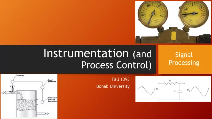
Instrumentation (and Signal Processing Process Control) Fall 1393 Bonab University Signal Processing - Introduction Signal Processing Analogue/digital filters: extensively used in sensor signal processing Pre-processing
Instrumentation (and Signal Processing Process Control) Fall 1393 Bonab University
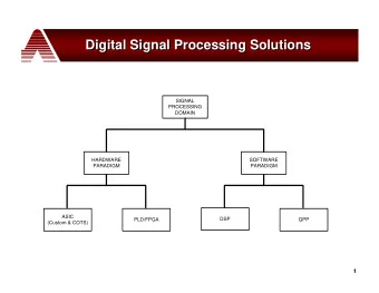
Signal Processing - Introduction Signal Processing • Analogue/digital filters: extensively used in sensor signal processing • Pre-processing • Post-processing • Analog filters: very common in dealing with: Aliasing phenomenon (acquisition) • Distortion: signal reconstructed from samples is different from the original continuous signal • Digital filters: generally used to post-process acquired signals + other sophisticated digital signal-processing techniques (say, Fast Fourier Transform to perform spectral analysis) • Analogue filter: analysis-synthesis • Passive components • Op-Amps • Digital: moving average (MA) and autoregressive moving average (ARMA) 2
Signal Processing - Introduction Signal Processing • Aliasing problem 3
Analog Filters Signal Processing • Two main reasons: • Buffer and reduce the impedance of sensors for interface with data acquisition • Eliminate high-frequency noise to prevent aliasing in ADC • Passive Analog • Few simple electronic components (resistors and capacitors) • Basic low-pass filter (Fig) used to remove (or attenuate) high-frequency noise • V o,1 may be very close to V i,1 , say 98% of this value, but V o,2 may be about 70% of V i,2 and so on… • Why? low-pass filter attenuates each signal according to its frequency 4
Analog Filters Signal Processing • precise amount of attenuation? 20 db /decade • frequency response (Bode plot) • Equation? Cutoff frequency • Kirchoff’s current law: _ Pass Band Stop Band • Laplace transform τ = RC, time-constant: time it takes for the filter to respond to a step input function by reaching 63% 1 τ = ω 𝐷 : Corner frequency • • Assuming sinusoidal inputs: ignoring the transient: 5
Analog Filters Signal Processing • Input-output relationship: _ _ • More standard form: _ _ • Higher frequencies (>> corner frequency of 10 r/s, Fig) high attenuation • Active Analog (Using Op-Amps) • Simple RC can be easily implemented • However since it is entirely passive: • Draw current from the input • And “load” the circuit connected to the output 6
Active Analog Filter (Using Op-Amps) Signal Processing • Op-amps eliminate this problem: • Current drawn from the input :very small (because op-amps internal resistances, of the order of 10 MO) • Likewise, as active devices, op-amps supply current to drive their output minimize the impact on any output circuit, such as DAQ card • So, Op-Amps & R & C = Active filter • Current Summation at inverting input: _ _ _ _ _ _ k τ _ _ Very similar to Passive (gain): Negative means min 180 o lag • K & τ : 2 DoF to adjust gain, corner-f independently 7
Active Analog Filter (in frequency domain) Signal Processing • The ratio of output to input voltage: _ • Bode: the same, with 20 log(k) shift up • Making the filter (usually): _ • Resistor (fixed/variable) • Capacitor (ceramic plate) • Op-Amp (say, LM741) • Designing the filter: • Choose corner-F (Better: measure) • 2 π f= 1/RC (1-equation, 2-un-known) • Choose a C (µF-pF) • Find R standardize • Choose another C if (not 1k-1M Ω ) • Keep in mind: tolerances 8
Other Active Signal Processing Circuits Signal Processing • Simple/complex tasks: • e.g. Adding two signals (say, for adjusting D.C offset) • Set v r = - D.C. offset _ • Generally: • Need: remove high-frequency noise in the signal before sampling it with an A/D • Usual color coding in the circuit: • Red: positive supply • Black: ground • Blue: signal 9
Digital Filters Signal Processing • Uses discrete data points sampled at regular intervals (from sensor output) • e.g. accelerometer (vibration in a beam) • Digital filters rely: Digital • not only on the current value of the measured variable • but also on its past values (raw/filtered form) _ _ • Input Averaging Filter Extend to more complex filter Called Moving Average (MA): _ _ _ • Filter with Memory _ _ • Large α Current value of input has more weight • Small α Past filtered signal has more weight (normally, α <1) 10
Example (filter with memory): Signal Processing Simple averaging filter: • No single α is the best • But α =0.5 may be better • More similar to input pattern To fit the application: • Fine-tune it • • There are mathematical methods Choose it based on frequency response (as in analog) • More effective Digital Filters : (higher order) • Combination of MA • And Autoregressive MA (ARMA) • 11
Variable Conversion Elements Variable Conversion • Often: measurement sensors’ outputs = Voltage signal measured by: voltage indicating instruments • However, many cases: output ≠ voltage • translational displacements • changes in various electrical parameters: • Resistance • Inductance • Capacitance • Current • Variations in the phase / frequency of an a.c. electrical signal • So, how convert output of sensors with Non-Voltage form? • Variable conversion elements • Particularly important: bridge circuits 12
Bridge Circuits Variable Conversion • Output: voltage level that changes as the measured physical quantity changes • Accurate method of measuring: • Resistance • Inductance • Capacitance • Enable: detection of very small changes (about nominal value) • So, immense importance in measurement • Many transducers measuring physical quantities: output • Expressed as a change in • Resistance, inductance, or capacitance • Example: a displacement-measuring strain gauge • Bridge excitation: • DC: for resistance • AC: for inductance, or capacitance • Bridge type: • Null type: calibration purposes • Deflection types: used in closed loop automatic control 13
Null-Type d.c. Bridge (Wheatstone Bridge) Variable Conversion • 4 arms of the bridge: • Unknown resistance R u • 2 equal value resistors R 2 and R 3 • variable resistor R v (usually a decade resistance box) • A d.c. voltage V i : applied across the points AC • Resistance R v is varied voltage across points BD = zero • Null point is measured with a high sensitivity galvanometer • Normally (high impedance voltage-measuring instrument): • I m = 0 I 1 = I 3 & I 2 = I 4 • At the null-point: if R2=R3 Ru = Rv 14
Deflection-Type d.c. Bridge Variable Conversion • Null-type: tedious to use, but highly accurate • Main difference: variable resistance R v is replaced by • fixed resistance R 1 • (same value as the nominal value of unknown resistance Ru) • Relationship: • Simplify: high impedance voltage measurement • Nonlinear: _ • Easier to use (less accurate) preferred in general 15
Deflection-Type d.c. Bridge Variable Conversion • Example: • A certain type of pressure transducer (range 0 – 10 bar) • Consists of a diaphragm with a strain gauge • The strain gauge has a nominal resistance of 120 O (one arm) • Other 3 arms each having a resistance of 120 O • Instrument’s input impedance can be assumed infinity • To limit heating effects, gauge current < 30 mA • Maximum permissible bridge excitation voltage? • Sensitivity of the strain gauge = 338 mO/bar • maximum bridge excitation voltage is used • bridge output voltage when measuring a pressure of 10 bar? • Solution: • I1 = current flowing in path ADC: • Balance: R u = 120 V i = 7.2 • Pressure=10bar: Resistance change = 3.38 O R u = 123.38 V o = 50mv 16
Sensitivity of the bridge Variable Conversion • How to deal with the non-linear relationship? _ • Special case: δ Ru << nominal value of Ru _ • New voltage: This is Bridge Sensitivity _ • Such approximation (linearization) is valid for transducers such as strain gauges • However, many instruments (say, resistance thermometers) • are inherently linear themselves (at least over a limited measurement range) • exhibit large changes • Other actions to improve linearity: • A common solution: • Make: R 2 , R 3 > 10x R 1 , R u (nominal) • The effect can be seen in an example 17
Sensitivity of the bridge – (non-linearity) Variable Conversion • Example: • a platinum resistance thermometer: • Range of 0 – 50 o C • Resistance at 0 o C = 500 O • Resistance varies with temperature at the rate of 4 O/ o C • Over this range of measurement, the output characteristic itself is nearly perfectly linear • Assuming: • _ 0.424 _ 0.833 • Non-linear: 0.424 • From 0 – 25: Vo change = 0.455-0 = 0.455 • From 25 – 50: Vo change = 0.833-0.455 = 0.378 Now if R 2 ,R 3 0.409 And Vi=26.1 18
Sensitivity of the bridge – (non-linearity) Variable Conversion • In increasing the values of R2 and R3 • Also necessary to increase the excitation from 10 to 26.1 • To obtain the same output levels • In practical applications: Vi set at maximum • Consistent with limitation (heating) maximize the measurement sensitivity (V0/dRu relationship) • • If smart system is used, the importance of this non-linearity is decreased 19
Recommend
More recommend
Explore More Topics
Stay informed with curated content and fresh updates.
