Some notes on continuous time finance Basics: Instantaneous total - PDF document

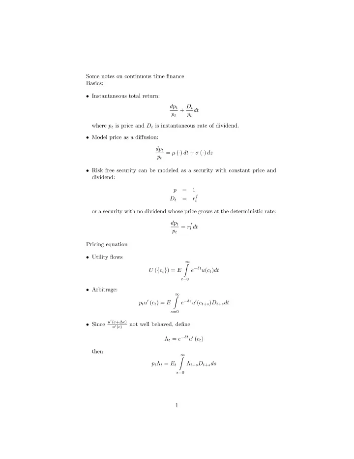
Some notes on continuous time finance Basics: • Instantaneous total return: dp t + D t dt p t p t where p t is price and D t is instantaneous rate of dividend. • Model price as a diffusion: dp t = µ ( · ) dt + σ ( · ) dz p t • Risk free security can be modeled as a security with constant price and dividend: p = 1 r f D t = t or a security with no dividend whose price grows at the deterministic rate: dp t = r f t dt p t Pricing equation • Utility flows ∞ � e − δt u ( c t ) dt U ( { c t } ) = E t =0 • Arbitrage: ∞ � p t u ′ ( c t ) = E e − δs u ′ ( c t + s ) D t + s dt s =0 • Since u ′ ( c +∆ c ) not well behaved, define u ′ ( c ) Λ t = e − δt u ′ ( c t ) then ∞ � p t Λ t = E t Λ t + s D t + s ds s =0 1

• Write this as s +∆ � p t Λ t = E t Λ t + s D t + s ds + E t p t +∆ Λ t +∆ s =0 + Λ t D t ∆ + E t p t +∆ Λ t +∆ • For small ∆ approximate integral as Λ t D t ∆ so that 0 = Λ t D t ∆ + E t ( p t +∆ Λ t +∆ − p t Λ t ) Now take ∆ → 0 0 = Λ t D t + E t [ d (Λ t p t )] • This is continuous time equivalent to p = E ( mx ) for return x and stochas- tic discount factor m . Risk premium • Ito’s Lemma implies d (Λ p ) = pd Λ + Λ dp + dpd Λ which for diffusions we can write as 0 = D � d Λ Λ + dp p + d Λ dp � P dt + E t Λ p • If p = 1 and D = r f t we have the risk-free rate equation d Λ t r f t dt = − E t Λ t • We can then get the risk-premium equation as � dp t � + D t � d Λ t dp t � dt − r f E t t dt = − E t p t P t Λ t p t CRRA: • Taylor series expansion: d Λ = − δe − δt dt + e − δt u ′′ ( c ) dc + 1 2 e − δt u ′′′ ( c ) dc 2 • Local curvature: − cu ′′ ( c ) γ = u ′ c ) γ ( γ + 1) = − c 2 u ′′′ ( c ) η = u ′ ( c ) so that 2 η dc 2 d Λ Λ = − δdt + γ dc c + 1 c 2 2

Risk premium with CRRA: • Risk free rate � dc 2 dc t − 1 � r f t t dt = δdt + γE t 2 ηE t c 2 c t t • Risk premium � dp t � + D t � dc t dp t � dt − r f E t t dt = γE t p t P t c t p t • Let dc = µ c cdt + σ c cdz then Sharpe-ratio satisfies µ p + D t P t dt − r f t dt ≤ γσ c σ p �� � 2 � dp t dp t where µ p = E t p t , σ p = E t p t Stochastic discount factor for stock with geometric brownian motion: • Assume stock value follows dS = µSdt + σSdz • Market completeness: all stochastic discount factors that price the stock S satisfy d Λ Λ = − rdt − ( µ − r ) dz − σ w dw σ where E ( dw dz ) = 0 Since dw uncorrelated we can set it to zero to price the asset. • Ito’s lemma implies � µ − 0 . 5 σ 2 � d ln S = dt + σdz � � r + 0 . 5 µ − r dt − µ − r d ln Λ = − dz σ σ Integrating these expression implies √ µ − 0 . 5 σ 2 � � ln S T = ln S o + T + σ Tε √ � � r + 0 . 5 µ − r T − µ − r ln Λ t = ln Λ o − Tε σ σ where ε = z t − z o √ ∼ N (0 , 1) T 3

European call option: • Let X denote strike price and S T denote stock value on expiration day. Payoff is C = max ( S T − X, 0) • Option value: � T Λ T C o = E t max ( S T − X, 0) Λ t 0 � ∞ Λ T = E t ( S T − X ) d f (Λ t , S T ) Λ t S T = X � ∞ Λ T = E t ( S T ( ε ) − X ) d f ( ε ) Λ t S T = X Deriving the Black-Scholes Formula: • Guess C = C ( S, t ) ie. function of price and time to expiration. • Ito’s Lemma: C t dt + C s dS + 1 2 C ss dS 2 dC = � C t + C s Sµ + 1 � 2 C ss S 2 σ 2 = + C s Sσdz • Asset pricing equation: 0 = E t ( d Λ C ) = CE t d Λ + Λ E t dC + E t d Λ dC Since d Λ E t Λ = − rdt we have 0 = − rC + C t + C s Sµ + 0 . 5 C ss S 2 σ 2 − S ( µ − r ) C s which gives the Black-Scholes Formula 0 = − rC + C t + SrC S + 1 2 C SS S 2 σ 2 Solution: • We are looking for a solution to 0 = − rC + C t + SrC S + 1 2 C SS S 2 σ 2 with boundary condition C = max [ S T − X, 0] 4

• Guess the solution satisfies: � � � � r + σ 2 / 2 r − σ 2 / 2 � � � � ln S o /X + T ln S o /X + T − Xe − rT Φ C o = S o Φ √ √ σ T σ T 5