1 SOME NOTES ON STATISTICAL INTERPRETATION Below I provide some - PDF document

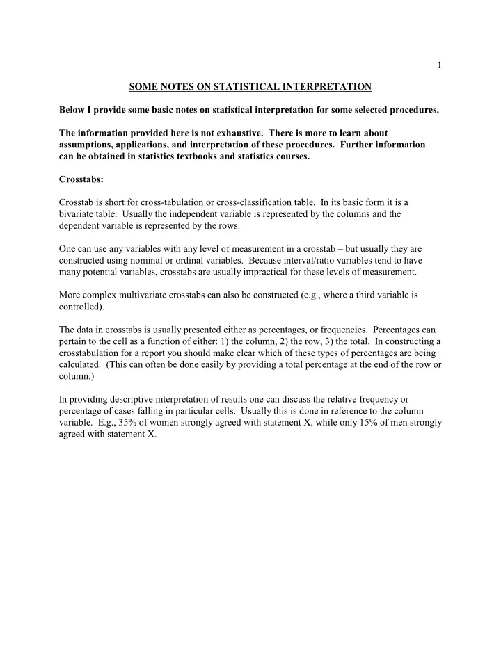
1 SOME NOTES ON STATISTICAL INTERPRETATION Below I provide some basic notes on statistical interpretation for some selected procedures. The information provided here is not exhaustive. There is more to learn about assumptions, applications, and interpretation of these procedures. Further information can be obtained in statistics textbooks and statistics courses. Crosstabs: Crosstab is short for cross-tabulation or cross-classification table. In its basic form it is a bivariate table. Usually the independent variable is represented by the columns and the dependent variable is represented by the rows. One can use any variables with any level of measurement in a crosstab – but usually they are constructed using nominal or ordinal variables. Because interval/ratio variables tend to have many potential variables, crosstabs are usually impractical for these levels of measurement. More complex multivariate crosstabs can also be constructed (e.g., where a third variable is controlled). The data in crosstabs is usually presented either as percentages, or frequencies. Percentages can pertain to the cell as a function of either: 1) the column, 2) the row, 3) the total. In constructing a crosstabulation for a report you should make clear which of these types of percentages are being calculated. (This can often be done easily by providing a total percentage at the end of the row or column.) In providing descriptive interpretation of results one can discuss the relative frequency or percentage of cases falling in particular cells. Usually this is done in reference to the column variable. E.g., 35% of women strongly agreed with statement X, while only 15% of men strongly agreed with statement X.

2 Chi-Square: Technically this is a “test of statistical independence”. That is, if two variable are unrelated then they are independent of one another. If not, they are dependent. Another way of thinking about this is that they are “associated”. Chi-square can be used with nominal and ordinal variables. If the significance value corresponding to the chi-square test is less than or equal to .05, then the test is deemed to be statistically significant and you can interpret the two variables in the test as being dependent – or associated. There are several limitations to the chi-square test. Two of these are: 1) the test does not tell you about the direction of an association (e.g., positive or negative), 2) the test does not tell you about the strength of an association. From the chi-square statistic (and its related level of significance) all you can say is that the variables are statistically associated or not. You can, however, try to interpret the percentages in the related crosstabulation. In Table 1, the chi-square is significant. This means that employment status and gender are statistically associated. The results in the crosstabulation suggest that men are more likely to be employed full-time.

3 Pearson’s Correlation: Pearson’s correlation is a bi-variate measure of association for interval/ratio level variables. Pearson’s correlation ranges from 0 to the absolute value of 1 (e.g. 1 or -1). A correlation of 0 means that there is no linear statistical association between two variables. A correlation of 1 means that there is a perfect positive correlation (or linear association) between two variables. A correlation of -1 means that there is a perfect negative correlation between two variables. A correlation of .50 means that there is a moderately strong positive correlation between two variables. There is also an associated test of significance. If the significance value (p.) is � .05, then the correlation is deemed to be statistically significant. In Table 2 the correlation between years of education and personal income is .42, and p. is < .01. Thus there is a significant, moderately strong positive correlation between education and income. (Another way of saying this is that there is a significant moderately strongly positive linear association between education and income.) In other words, people with higher levels of education tend to earn higher levels of income, people with lower levels of education tend to earn lower levels of income.

4 Multiple Regression Analysis. Multiple regression analysis examines the strength of the linear relationship between a set of independent variables and a single dependent variable (measured at the interval/ratio level). 2 The R provides the proportion of variation in the dependent variable that is explained by the independent variables in the model. For example, the independent variables in Model 5 of Table 7 explain .20 of the variation in environmentally friendly behaviour, or, converted into a percentage, they explain 20% of the variation in environmentally friendly behaviour. There are two types of coefficients that are typically be displayed in a multiple regression table: unstandardized coefficients, and standardized coefficients. To interpret an unstandardized regression coefficient: for every metric unit change in the independent variable, the dependent variable changes by X units. For instance, if income is the dependent variable, and years of education is one of the independent variables, and the unstandardized regression coefficient for education is 3,000, then this would mean that for every additional year of education a respondent has, their income increases by $3,000.00 (controlling for the other independent variables in the equation). In multiple regression, the effects of the independent variables are always net effects – controlling simultaneously for the effects of the other variables in the equation. One advantage of using unstandardized coefficients is that they have readily interpretable substantive meaning (such as in the example of education and income given above). One disadvantage is that the independent variables usually have different metrics (e.g. income in dollars, age in years, attitudes on a rating scale, etc.). This makes it difficult to compare the relative influence of different independent variables upon the dependent variable. Standardized regression coefficients are based on changes in standard deviation units. For example, in Model 5 of Table 7, for every standard deviation unit increase in activism, the respondent’s score on the environmentally friendly behaviour index increases by .18 standard deviation units.

5 One advantage of using standardized regression coefficients is that you can compare the relative strength of the coefficients. Generally, the closer to the absolute value of 1 the coefficient is, the stronger the effect of that independent variable on the dependent variable (controlling for other variables in the equation). The closer the coefficient is to 0, the weaker the effect of that independent variable. For example, in Model 1 of Table 1, Age has the strongest effect on environmentally friendly behaviour (-.23), while income (log) has the smallest effect (-.08). (0 means no net effect; under unusual circumstances in multiple regression, standardized regression coefficients can be greater than the absolute value of 1; in bivariate regression the standardized regression coefficient – also known as Pearson’s Correlation Coefficient – has a maximum value of the absolute value of 1.) Usually independent variables are measured at the interval/ratio level. While it is technically not supposed to be done, sometimes ordinal variables (measured in likert- type scales) are treated as interval/ratio level variables and used as independent variables. It is also possible to include categorical variables as independent variables – but they have to be binarized, and coded as 0 or 1. Also, at least one category has to be left out to serve as a reference category. Variables coded in this way are referred to as dummy variables. For example, in Table 7 gender is coded as male = 1, and female = 0. If one had income as a dependent variable in a multiple regression, and the unstandardized regression coefficient for gender was 10,000 then (assuming the previous coding scheme) men would make 10,000 more than women – controlling for other variables in the equation. Another example in Table 7 is “Gendpar” where female parents are coded as 1, and everyone else is coded as 0. It is somewhat more difficult to interpret standardized regression coefficients for dummy variables because standard deviation unit changes are somewhat meaningless when there are only two categories. In Model 1 of Table 7, it can be said that there is a significant effect for gender, females have higher scores for environmentally friendly behaviour. In multiple regression analysis, significance levels are usually also reported that are associated with the individual regression coefficients, and also a separate significance level is reported for 2 the equation as a whole and associated with the R .