Small FPGA-Based Multiplication-Inversion Unit for Normal Basis over GF ( 2 m ) Métairie Jérémy, Tisserand Arnaud and Casseau Emmanuel CAIRN - IRISA July 9 th , 2015 ISVLSI 2015 PAVOIS ANR 12 BS02 002 01 1 / 19
Summary Elliptic Curves Background and State-of-the-Art 1 Proposed Solution 2 Architecture and Figures 3 2 / 19
Elliptic Curves Elliptic Curves E = { ( x , y ) ∈ GF ( p ) 2 such that y 3 = x 3 + a · x + b } Equation: y 2 = x 3 + 3 x + 5 in Point Operations GF ( 1223 ) [ k ] P = P + P + . . . + P � �� � k times ADD : R = P + Q with P � = Q and R , P , Q ∈ E DBL : R = P + P with R , P ∈ E Discrete Logarithm Problem Knowing P and Q it is very hard to find k ∈ Z such Q = [ k ] P 3 / 19
Double-And-Add vs. Halve-and-Add Algorithms Inputs: P ∈ E and k = Inputs: P ∈ E and k = ( k 0 , k 1 , . . . , k m − 1 ) ∈ N ( k 0 , k 1 , . . . , k m − 1 ) ∈ N Output: Q = [ k ] P Output: Q = [ k ] P 1: Q ← O 1: Q ← O 2: for i from 0 to m − 1 do 2: for i from 0 to m − 1 do if k i = 1 then if k i = 1 then 3: 3: Q ← Q + P Q ← Q + P 4: 4: end if end if 5: 5: P ← 2 · P P ← P / 2 6: 6: 7: end for 7: end for 8: return Q 8: return Q Double and Add Faster Computation Protection against (some) Halve and Side Add Double and Halve and Channel Attacks Add Add 4 / 19
Elliptic Curves over GF ( 2 m ) Definition E = { ( x , y ) ∈ GF ( 2 m ) 2 such that y 2 + x · y = x 3 + a 2 · x 2 + a 6 } Let P = ( x p , y p ) and Q = ( x q , y q ) be two points in E . One can compute R = P + Q as follows (affine coordinates): λ = x p + x q y p + y q then x r = λ 2 + λ + x p + x q + a and y r = λ · ( x p + x r ) + x r + p y 1 - Note that y p + y q is costly to compute ( ≈ 10 multiplications) - Recommended m ∈ { 163 , 233 , 283 , 409 , 571 } 5 / 19
Normal Basis (NB) Every element A ∈ GF ( 2 m ) can then be written as follows: m − 1 a i β 2 i with a i ∈ { 0 , 1 } � A = i = 0 Note that element A can be stored as a vector a = [ a 0 , a 1 , . . . , a m − 1 ] . 1 0 0 0 0 0 0 0 1 Square-root (Circular Right Shift) Square (Circular Left Shift) 0 0 0 0 0 0 0 1 1 ⇒ Easy squares but more complicated multiplications. 6 / 19
Massey-Omura Multiplication in Binary Finite Field. [4] Inputs: A ∈ GF ( 2 m ) (NB), B ∈ GF ( 2 m ) (NB) CTRL Output: P = A · B (NB) m 1: P ← 0 ; i ← 0 2: while i < m do P [ 0 ] ← A · M 0 · ( B ) T 3: m i ← i + 1 4: A ← LeftShift ( A , 1 ) 5: m B ← LeftShift ( B , 1 ) 6: P ← LeftShift ( P , 1 ) 7: 8: end while 1 9: return P 7 / 19
Fermat’s Little Theorem Fermat’s Little Theorem For any α ∈ GF ( 2 m ) ∗ α − 1 = α 2 m − 2 If one wants to compute α 2 10 − 2 = α ( 1 111 111 110 ) 2 , one can perform the following operations : P 0 = α ( 1 ) 2 Itoh-Tsujii Sequence [3] 0 · P 0 = α ( 10 ) 2 · α ( 1 ) 2 = α ( 11 ) 2 P 1 = P 2 P 2 = P 2 2 1 · P 1 = α ( 1100 ) 2 · α ( 11 ) 2 = α ( 1111 ) 2 P 3 = P 2 4 2 · P 2 = α ( 11110000 ) 2 · α ( 1111 ) 2 = α ( 11111111 ) 2 3 · P 0 = α ( 1111111110 ) 2 · α ( 1 ) 2 = α ( 111111111 ) 2 P 4 = P 2 4 = α 2 10 − 2 = α ( 1 111 111 110 ) 2 P 5 = P 2 Here, only 4 multiplications are necessary to perform the whole exponentiation (8 for square-and-multiply algorithm). 8 / 19
Using Symmetries in the Massey-Omura Algorithm [4] For the special multiplication case B = A 2 j , a symmetry appears. Let us consider an example where A = [ a 0 , a 1 , a 2 ] and B = [ a 2 , a 0 , a 1 ] . The different steps of the regular Massey-Omura algorithm: a 2 � � Step 1 : p 0 = a 0 a 1 a 2 · M 0 · a 0 a 1 a 0 � � Step 2 : p 1 = a 1 a 2 a 0 · M 0 · a 1 a 2 a 1 � � Step 3 : p 2 = a 2 a 0 a 1 · M 0 · a 2 a 0 9 / 19
Using Symmetries in the Massey-Omura Algorithm [4] For the special multiplication case B = A 2 j , a symmetry appears. Let us consider an example where A = [ a 0 , a 1 , a 2 ] and B = [ a 2 , a 0 , a 1 ] . The different steps of the regular Massey-Omura algorithm: a 2 � � Step 1 : p 0 = a 0 a 1 a 2 · M 0 · a 0 a 1 a 0 � � Step 2 : p 1 = a 1 a 2 a 0 · M 0 · a 1 a 2 a 1 � � Step 3 : p 2 = a 2 a 0 a 1 · M 0 · a 2 a 0 9 / 19
Proposed Multiplication Algorithm when gcd ( j , m ) = 1 Inputs: A ∈ GF ( 2 m ) (NB) , B ∈ GF ( 2 m ) such that B = A 2 j (NB) and j ∈ N Output: P = A · B in normal basis 1: C ← LeftShift ( B , m − j ) 2: P ← 0 3: i ← 0 4: while i < ⌈ m / 2 ⌉ do g ← M 0 · ( A ) T 5: P [ j ] ← g · ( C ) T ; P [ 0 ] ← g · ( B ) T 6: A ← LeftShift ( A , 2 j ) ; B ← LeftShift ( B , 2 j ) ; C ← LeftShift ( C , 2 j ) 7: P ← LeftShift ( P , 2 j ) i ← i + 1 8: 9: end while 10: return P Different j values may be used for the exponentiation process. In hardware, variable shifters are area costly for large operands ⇒ We need to remove those 2 j shifts. 10 / 19
Proposed Multiplication Algorithm with θ Constant Inputs: A ∈ GF ( 2 m ) (NB) , B ∈ GF ( 2 m ) such that B = A 2 j (NB) and j ∈ N , θ ∈ N Output: P = A · B in normal basis 1: C ← LeftShift ( B , m − j ) 2: P ← 0 3: i ← 0 4: while i < ⌈ N ( j , θ ) ⌉ do g ← M 0 · ( A ) T 5: P [ j ] ← Tmp · ( C ) T ; P [ 0 ] ← Tmp · ( B ) T 6: A ← LeftShift ( A , θ ) ; B ← LeftShift ( B , θ ) ; C ← LeftShift ( C , θ ) 7: P ← LeftShift ( P , θ ) i ← i + 1 8: 9: end while 10: return P N ( j , θ ) is the number of iterations to get all the bits of P . Note that N ( j , θ ) ≥ ⌈ m / 2 ⌉ . 11 / 19
A Wise Choice of the Constant Shift θ The goal is now to find θ which minimizes D = � i ∈I N ( i , θ ) where I is the set of all the j implied in the computations of the A 2 j · A patterns used in the exponentiation (inversion). θ D m 163 72 732 233 36 1046 283 28 1431 409 35 2263 571 171 3221 Definition Permuted Normal Basis (PNB) representation where element A = [ a 0 , a 1 , a 2 , . . . , a m − 1 ] is represented by A ′ = [ a 0 , a θ , a 2 θ mod m , . . . , a ( m − 1 ) θ mod m ] . 12 / 19
Shifting Through BRAMs We duplicate w times the bits of P = A · B = [ p 0 , p 1 , . . . , p m − 1 ] in a BRAM using the following patterns: p 1 p 2 p 3 p 0 p 1 p 2 BRAM p 1 p 2 p 3 1 p 0 , p 1 , . . . , p w − 1 p 0 p 1 p 4 p 1 , p 2 , . . . , p w p 2 p 3 p 4 . . . p 3 p 4 p 0 p m − 1 , p 3 , . . . , p m − w − 2 p 4 p 0 p 1 2 BRAMs in recent FPGAs are large enough to support the m · w bits (18 Kb on a low-cost Spartan-6 and Virtex 4). 13 / 19
Architecture: Multiplier CTRL m ROL REGISTER A m m m m ROL REGISTER B ROL REGISTER C w w 14 / 19
Architecture: Multiplication-Inversion Unit (MIU) Input B w CTRL MUX2 w w w Massey REG1 w w REG2 2 Omura Output w Multiplier w l P or R w MUX1 l l w Input A 1 2 l 2 w Implementation of the Multiplication-Inversion Unit on Virtex-4 LX100 with w = 32 and ℓ = 10. m Algo. Area Freq. Inv. Time Slices (LUT, FF) MHz µ s MO1 [5]* 3378 (5615, 2016) 125 64 . 4 571 RM2 [6]* 4976 (9445, 2090) 107 38 . 7 our PNB 4308 (5928, 2650) 125 47 . 7 Hybrid ( d = 13) [1] #LUTs = 85268 74 4 . 98 571 Parallel ( d = 13) [2] #LUTs = 56657 82 5 . 00 15 / 19
Implementation Results Hardware implementation on on Virtex-4 LX100 and time estimation of a scalar multiplication ( m = 571) only using the Halve-and-Add algorithm. Algorithm halving area ATP · 10 − 3 ms #LUTs MO1 [5]* 17 . 3 5742 95 RM2 [6]* 13 . 0 9572 122 NAF our PNB 14 . 3 6055 82 Parallel IT (d=13) [2] 1 . 59 56784 90 Hybrid IT (d=13) [1] 1 . 60 85395 136 MO1 [5]* 14 . 6 79 RM2 [6]* 8 . 95 76 3-NAF our PNB 11 . 3 similar 65 Parallel IT (d=13) [2] 1 . 34 74 1 . 40 Hybrid IT (d=13) [1] 119 ATP: area-time product 16 / 19
Conclusion We proposed a new Multiplication-Inversion Unit that Uses a new normal basis representation (PNB) ⇒ replacement of large shifters by BRAMs Is ≈ 20 % faster than classical MO approach for halving-based scalar multiplication We still have to : Have a full implementation of a crypto-processor Study security aspects of our design Thank you for your attention ! 17 / 19
References [1] R. Azarderakhsh, K. Jarvinen, and V. Dimitrov. Fast inversion in GF(2 m ) with normal basis using hybrid-double multipliers. IEEE Trans. Comp. , 63(4):1041–1047, April 2014. [2] J. Hu, W. Guo J. Wei, and R.C.C. Cheung. Fast and generic inversion architectures over GF(2 m ) using modified Itoh-Tsujii algorithms. IEEE Transactions on Circuits and Systems II: Express Briefs , 2015. Accepted paper. [3] Itoh and Tsujii. A fast algorithm for computing multiplicative inverses in gf(2m) using normal bases. Information and Computation , 1988. [4] Omura Massey. Computational method and apparatus for finite field arithmetic. U.S. Patent Application , 1981. [5] J. K. Omura and J. L. Massey. Computational method and apparatus for finite field arithmetic. US Patent US4587627 A, May 1986. [6] A. Reyhani-Masoleh. Efficient algorithms and architectures for field multiplication using Gaussian normal bases. IEEE Trans. Comp. , 55(1):34–47, 2006. 18 / 19
Recommend
More recommend
Unleash a World of Digital Possibilities—Browse, Share, and Explore Content Without Boundaries