Signal Processing General Introduction Based Intrusion Detection - PDF document

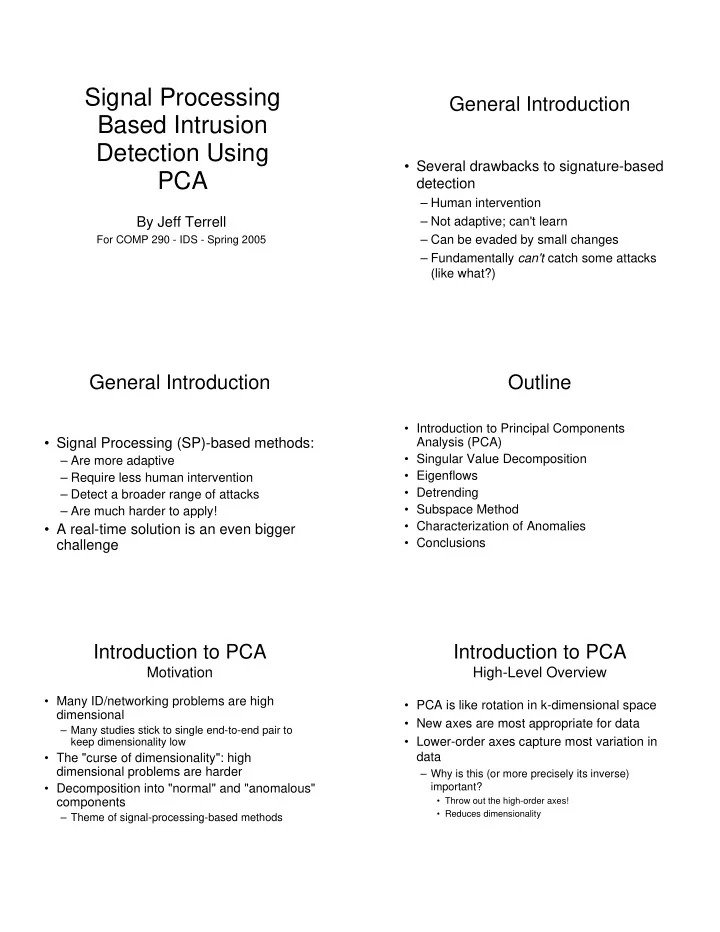
Signal Processing General Introduction Based Intrusion Detection Using • Several drawbacks to signature-based PCA detection – Human intervention By Jeff Terrell – Not adaptive; can't learn For COMP 290 - IDS - Spring 2005 – Can be evaded by small changes – Fundamentally can't catch some attacks (like what?) General Introduction Outline • Introduction to Principal Components • Signal Processing (SP)-based methods: Analysis (PCA) • Singular Value Decomposition – Are more adaptive • Eigenflows – Require less human intervention • Detrending – Detect a broader range of attacks • Subspace Method – Are much harder to apply! • Characterization of Anomalies • A real-time solution is an even bigger • Conclusions challenge Introduction to PCA Introduction to PCA Motivation High-Level Overview • Many ID/networking problems are high • PCA is like rotation in k-dimensional space dimensional • New axes are most appropriate for data – Many studies stick to single end-to-end pair to • Lower-order axes capture most variation in keep dimensionality low data • The "curse of dimensionality": high dimensional problems are harder – Why is this (or more precisely its inverse) important? • Decomposition into "normal" and "anomalous" components • Throw out the high-order axes! • Reduces dimensionality – Theme of signal-processing-based methods

Introduction to PCA Introduction to PCA 2-D example [1] Intuitive Examples • Football - 1 st axis along the length • Piece of paper - "intrinsically" ~2D • Faces - A 100x100 bitmap is 10,000D, but how many dimensions would we need optimally? – Answer: 42 Introduction to PCA Introduction to PCA Geometric Details Demonstrations • 1 st axis captures greatest variation • http://www.uwlax.edu/faculty/will/svd/pe – In 2-D, what will the 1 st axis be? rpframes/index.html • 2 nd axis captures greatest remaining variation • http://www.cac.sci.kun.nl/people/philipg/ – Remove 1 st axis by "collapsing" data points into nfo-6/ orthogonal (hyper) plane • Rinse and repeat • All axes must be orthogonal – Last axis is easy • End result: rotation in k-D space Setup (from [2]) Setup (from [2]) • Abilene traffic data used • Measurement is the number of flows • 11 Points of Presence (PoPs) • Thus X is 2016x121 data matrix – Column i is timeseries of i -th OD flow • 11^2 = 121 Origin-Destination (OD) flows – Row j is vector of measurements at j -th interval • Aggregation at 5 minutes for 1 week • Note the high dimensionality (121D) (2,016 intervals)

Singular Value Decomposition Singular Value Decomposition • Any matrix can be decomposed into 3 • An eigenflow, U i , is a 2016-vector, and matrices: U*S*V T there are 121 of them • V T , 121x121, is PCA's rotation matrix (a • Each U i is a component of the data frame ) • Each OD-flow timeseries can be • S, 121x121, is diagonal and contains completely represented with a ordered singular values � k weighted sum of eigenflows – The weights are given in V T • U, 2016x121, contains our eigenflows Singular Value Decomposition SVD - Scree Plots • Recall: S, diagonal, contains � 1 - � 121 • A scree plot is a plot of i vs. � i 2 • � i 's are arranged in decreasing order • Useful for portraying relative • They are sqrt(eigenvalues) of V*V T importance of each � i • They represent amount of energy explained by component i – What does this say about our eigenflows? • They are arranged in decreasing order of importance SVD - Scree Plots SVD - Recap • X = U*S*V T • U i = column of U = eigenflow • S, diagonal, is singular values � i • V T is PCA's rotation matrix • Singular Value i represents amount of energy captured by U i

A Taxonomy of Eigenflows A Taxonomy of Eigenflows D-eigenflow example • Deterministic (D-) eigenflows – Large trends – Periodic – Defined heuristically as having maximum frequency component at 12 or 24 hours A Taxonomy of Eigenflows A Taxonomy of Eigenflows • Spike (S-) eigenflows • Noise (N-) eigenflows – Major element is at least 1 large spike – Resembles Gaussian noise – Defined heuristically as having at least 1 – Think of these as making up the leftover value more than 5 standard deviations energy from the mean – Defined heuristically with a qq-plot A Taxonomy of Eigenflows A Taxonomy of Eigenflows • Where are we going with this? – We can now decompose each OD flow in terms of how deterministic, spiky, or noisy it is – Detrending – Forecasting

A Brief Note on Stability Discussion • Detrending: remove D-eigenflows from an OD flow • Why would thresholding alone fail to – Now the timeseries is stable , so we can use detect anomalies? simple thresholding to detect anomalies – We'd never detect an anomaly at 4 A.M. • Forecasting: use most significant eigenflows – We'd detect lots of anomalies at noon of one trace to predict, say, next week's traffic – Identify anomalies this way • The timeseries is not stable ...yet Introduction to Discussion the Subspace Method (from [3]) Or, do both at the • Very similar to detrending same time! – Separation of "normal" from "anomalous" • Mark first eigenflow with a value > 3 standard deviations from the mean • This is the beginning of the "anomalous subspace" • Everything prior is the "normal subspace" Application of Introduction to Subspace Method the Subspace Method • Each OD-flow is completely characterized by normal and anomalous components • So, we can remove the normal components, and examine the residuals

Applying the Applying the Subspace Method Subspace Method • Similar to detrending, we can now just • Let N be projection of data onto normal threshold on A to detect anomalies subspace (the modeled part) – Project each 121-D point onto A • Let A be projection onto anomalous – How could we tell how anomalous this projection subspace (the residual part) is? • Euclidean distance from origin • Heavy on statistics, but confidence intervals and such are involved Discussion Setup (from [4]) • False positive rate and detection rate • Same setup as before – False positive rate estimated with EWMA • Except, now perform subspace method and other techniques on byte, packet, and flow matrices – Detection rate estimated by injecting • Objective: after detection, characterize anomalies (and quantify) anomalies • Feasibility of deployment onto actual networks Setup (from [4]) Characterization of Anomalies • We've seen how to catch anomalies by • By detecting coinciding anomalies in thresholding residuals bytes, packets, and flows, can crudely classify the type of anomaly • This time, also catch anomalies in normal subspace with use of the t 2 – Coinciding spike in bytes & packets may mean large transfer statistic – Coinciding spike in flows & packets might be a network scan

Characterization of Anomalies Discussion • By also checking for dominant sources • How might we distinguish between or destinations, we can do better DDoS attack and flash crowd? – DDoS is manifest as spike in F, P, or FP – Paper says flash crowds usually counts with a dominant destination dominated by a single OD-flow – Most worms will manifest as spike in F • Even without bulletproof counts with a dominant port characterization, this is still a big help to network administrators Concluding Remarks Concluding Remarks • PCA and the subspace method are • PCA and the subspace method are not better in many ways than signature- the only signal-processing based based means of detection methods of intrusion detection – Adaptive • Others include: – No human intervention – Spectral analysis • However, there are still plenty of – Wavelet decomposition improvements to be made – Other SVD techniques Questions? 1. http://www.mech.uq.edu.au/courses/mech4710/pca/s1.htm 2. "Structural Analysis of Network Traffic Flows" by A. Lakhina, K. Papagiannaki, M. Crovella, C. Diot, E. Kolaczyk, and N. Taft 3. "Diagnosing Network-Wide Traffic Anomalies" by A. Lakhina, M. Crovella, and C. Diot 4. "Characterization of Network-Wide Anomalies in Traffic Flows" by A. Lakhina, M. Crovella, and C. Diot