Exploratory Data Analysis (or Searching for Stationarity) When an - PowerPoint PPT Presentation

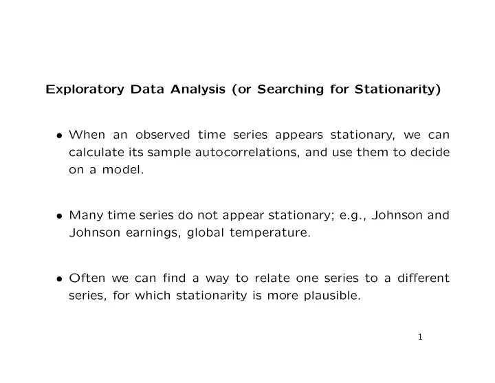
Exploratory Data Analysis (or Searching for Stationarity) • When an observed time series appears stationary, we can calculate its sample autocorrelations, and use them to decide on a model. • Many time series do not appear stationary; e.g., Johnson and Johnson earnings, global temperature. • Often we can find a way to relate one series to a different series, for which stationarity is more plausible. 1

Trends and Detrending • Some series can be modeled as x t = µ t + y t , where y t is stationary. • If µ t is a parametric form, we can estimate it and subtract it. That is, we use the residuals from a fitted trend. • The form of trend might be linear, or higher degree polyno- mial, or some other function suggested by theory. 2

Example: 20 th Century Global Temperature lmg1900 = lm(g1900 ~ time(g1900)); plot(ts(residuals(lmg1900), start = 1900)); 0.3 Residuals 0.0 −0.3 1900 1920 1940 1960 1980 2000 Time 3

Differencing • Some series still appear nonstationary after detrending. • E.g. the “trend” µ t is a random walk with drift: t � µ t = δt + w j j =1 Here E( x t ) = δt , but t � x t − E( x t ) = w j + y t j =1 with a variance that grows with time. 4

• But now the first differences ∇ x t = x t − x t − 1 = δ + w t + y t − y t − 1 are stationary. • Define the backshift operator B by Bx t = x t − 1 • Then ∇ x t = (1 − B ) x t . • Also second differences ∇ 2 x t = (1 − B ) 2 x t = x t − 2 x t − 1 + x t − 2 , etc. Easy for any positive integer d ; possible for fractional d . 5

Example: 20 th Century Global Temperature plot(diff(g1900)); 0.3 diff(g1900) 0.0 −0.3 1900 1920 1940 1960 1980 2000 Time • Both detrending and differencing give apparently stationary results. 6

acf(diff(g1900)); Series diff(g1900) 1.0 ACF 0.4 −0.2 0 5 10 15 Lag • Differencing has removed almost all auto-correlation. 7

acf(residuals(lmg1900)) Series residuals(lmg1900) 1.0 ACF 0.4 −0.2 0 5 10 15 Lag • Removing the trend without differencing leaves more auto- correlation. 8

Transformation (Re-expression) • Some series need to be re-expressed. • Most commonly logarithms, sometimes square roots (espe- cially with counted data). • Often re-expression improves stationarity, and other desirable features such as symmetry of distribution. • E.g. Glacial varve thicknesses, Johnson and Johnson earn- ings. 9

Periodic Signals • If a series is plausibly modeled as a cosine wave plus noise, we can fit x t = A cos(2 πωt + φ )+ w t = ( A cos φ ) cos(2 πωt ) − ( A sin φ ) sin(2 πωt ) by least squares. • If ω is known (e.g., ω = 1 / 12 for an annual cycle in monthly data), this is a linear regression: x t = β 1 cos(2 πωt ) + β 2 sin(2 πωt ) 10

• If ω is of the form j/n for integer j ( n = series length), then n β 1 = 2 ˆ � x t cos(2 πtj/n ) , n t =1 n β 2 = 2 ˆ � x t sin(2 πtj/n ) . n t =1 • For other ω , use standard linear least squares regression. • If ω is unknown, either: β 1 ( j/n ) 2 + ˆ β 2 ( j/n ) 2 – try all ω s of the form j/n , plotting ˆ against j/n (the periodogram ); – use non-linear least squares for other ω . 11

# detrend global temperature using a quadratic fit gtres = residuals(lm(globtemp ~ time(globtemp) + I(time(globtemp)^2))); gtres = ts(gtres, start = start(globtemp)); par(mfcol = c(2, 1)); plot(gtres); # use spectrum() to plot the periodogram of detrended global temperature spectrum(gtres, log = "no"); 12

Smoothing a Time Series • Smoothing a time series makes long-term behavior (low fre- quencies) more apparent. E.g. global temperature, Johnson and Johnson earnings. • Many types of smoother: – moving averages; – kernel smoothers; – lowess, supsmu, etc.; – smoothing splines. 13

# Trailing yearly average J&J earnings plot(jj) lines(filter(jj, rep(1, 4)/4, sides = 1), col = "red") title("Trailing 4-quarter averages") # smooth global temperatures over a 30 year window # (note half weight on end values) plot(globtemp) lines(filter(globtemp, c(.5, rep(1, 29), .5)/30), col = "red") title("Centered 30 year averages") 14

Smoothing a Scatter Plot • Smoothing a scatter plot can also reveal behavior. • E.g. daily NYSE returns plotted against previous day. 15

# scatter plot of NYSE return against previous day, # with lowess smooth plot(nyse[-length(nyse)], nyse[-1], xlim = c(-0.02, 0.02), ylim = c(-0.02, 0.02)) lines(lowess(nyse[-length(nyse)], nyse[-1], f = 1/5), col = "red") title("NYSE daily return against previous day") 16