Chapter 5 Searching and Binary Search Trees 5.1 Searching sequence - PowerPoint PPT Presentation
CS 2412 Data Structures Chapter 5 Searching and Binary Search Trees 5.1 Searching sequence The purpose of searching : find out some specific item from a collection of data. Key of information: some kind of index of items in the collection of
CS 2412 Data Structures Chapter 5 Searching and Binary Search Trees
5.1 Searching sequence The purpose of searching : find out some specific item from a collection of data. Key of information: some kind of index of items in the collection of data. External and internal searching: external searching used for search from databases. Here we basically consider algorithms for internal searching. Key type usually are simple: usually int, float, char * Data Structure 2015 R. Wei 2
macro substitution with parameters: macro substitution can adding parameters. Example: #define GETBIT(w,n) (((unsigned int) (w) >> (n)) & 01) The source code: GETBIT(15,2) will be replaces with (((unsigned int) (15) >> (2)) & 01) Note: >> n moves right n bits. The extra parentheses of w, n are necessary. Otherwise might cause problems if w is an expression. Data Structure 2015 R. Wei 3
In searching, we need to define equality and less than of keys. #define EQ(a,b) ((a)==(b)) #define LT(a,b) ((a)<(b)) For characters: #define EQ(a,b) (!strcmp((a),(b))) #defing LT(a,b) (strcmp((a),(b))<0) Data Structure 2015 R. Wei 4
Sequential search Consider sequential search in a list implemented by an array. The ListEntry contains a KeyType key . int SequentialSearch(List list,KeyType target) { int location; for(location=0;location<list.count;location++) if(EQ(list.entry[location].key,target)) return location; return -1; } Data Structure 2015 R. Wei 5
5.2 Complexity analysis and big- O notation If an algorithm is linear, i.e., there is no loops, then its efficiency is a function of the number of instructions it contains. On the other hand, functions that use loops or recursion vary widely in efficiency. So we will focus on loops. Linear loops examples: for (i = 0; i< n; i++) application code for (i = 0; i< n; i += 2) application code The complexity of above loops are proportional of n , denoted O ( n ) Data Structure 2015 R. Wei 6
Logarithmic loops: for (i = 0; i< n; i *=2) application code The complexity of the above loop is proportional of log 2 n , denote O (log n ) for (i = 0; i< n; i++) for( j = 1; j<=n; j*=2) application code The complexity of the above nested loop is proportional of n log 2 n , denoted O ( n log n ). Data Structure 2015 R. Wei 7
for (i = 0; i< n; i++) for (j = 1; j < n; j++) application code The complexity of the above nested loop is proportional of n 2 , denoted O ( n 2 ). Here we just gave some description of big- O notation, but not the formal definition. Basic complexity: O (log n ) , O ( n ) , O ( n log n ) , O ( n 2 ) , O ( n k ) , O ( c n ) , and O ( n !). Data Structure 2015 R. Wei 8
The complexity of sequential search The most time consuming in the program is comparing. Suppose the size of the list is n . In average, how many compares need for the program? 1 + 2 + 3 + · · · + n n. This equals to: n ( n + 1) = 1 2( n + 1) . 2 n So it is proportional to n , O ( n ). Data Structure 2015 R. Wei 9
Testing can also used to estimate CPU time. In a test, a sample data is set up. Then run the program and count the CPU time used. We will assume the search is in random. int RandomInt(int low, int high) { if(low > high) Error("RandomInt: low cannot be greater than high."); return(high - low +1)*(rand()/(double)INT_MAX)+low; } Data Structure 2015 R. Wei 10
#include<time.h> float Time(int flag) { static clock_t start; clock_t end; if(flag==START){ start=clock(); return 0.0; }else{ end=clock(); return (end-start)/CLK_TCK; } } Data Structure 2015 R. Wei 11
void TestSearch(List list,int (*Search(List list, KeyType target), int searchcount) { float elapsedtime; extern long compcounter; /*global comparison counter*/ ...... (void)Time(START); ...... for(i=0;i<serchcount;i++){ target=2*RandomInt(1,list.count)-1; if(Search(list,target)==-1) printf("%d not found\n",target); } ...... elapsdtime=Time(END); ...... Data Structure 2015 R. Wei 12
Binary sequential search If the keys of a list are arranged in order, then we can use a very efficient search method: binary sequential search. In that case, only n times comparisons are needed for search a list of length 2 n . Definition An ordered list is a list in which each entry contains a key, such that the keys are in order. That is, if entry i comes before entry j in the list, then the key of entry i is less than or equal to the key of entry j . Data Structure 2015 R. Wei 13
/*insert resulting an ordered list*/ void InsertOrder(List *list,ListEntry x) { int current; ListEntry currententry; for(current=0;current<ListSize(*list);current++){ currententry=RetrieveList(*list,current); if(LE(x.key,currententry.key)) break; } InsertList(list,x,current); } Data Structure 2015 R. Wei 14
In binary search algorithms, we use two indices top and bottom , such that the target is between the two indices. The key of top is greater than or equal to the key of index bottom . Main idea: compute middle=(top+bottom)/2 and compare the key at middle with target . Then move the top or bottom to middle . The binary search process terminates when top <= bottom . The complexity of binary search for ordered sequence is O (log n ). Data Structure 2015 R. Wei 15
Asymptotics Asymptotics is an important concept to compare the efficiency of computer algorithms. Definition If f ( n ) and g ( n ) are functions defined for positive integers, then to write f ( n ) is O ( g ( n )) means that there exists a constant c such that | f ( n ) | ≤ c | g ( n ) | for all sufficient large positive integers n . Example. If f ( n ) = 4 n + 200, then f ( n ) is O ( n ). If f ( n ) = 0 . 001 n 2 , then f ( n ) is not O ( n ), but O ( n 2 ). Data Structure 2015 R. Wei 16
If f ( n ) is a polynomial in n with degree r , then f ( n ) is O ( n r ), but is not O ( n s ) for any s < r . Any logarithm of n grows more slowly (as n is increases) than any positive power of n . Hence log n is O ( n k ) for any k > 0, but n k is never O (log n ) for any power k > 0. If f ( n ) − g ( n ) is O ( h ( n )), then we define f ( n ) = g ( n ) + O ( h ( n )). Running time for successful search a list of length n : • Sequential search is 1 2 n + O (1). • Binary search is 2 lg n + O (1). • Retrieval from a contiguous list is O (1). Most common orders: O (1) , O (log n ) , O ( n ) , O ( n log n ) , O ( n 2 ) , O ( n 3 ) , O (2 n ) Data Structure 2015 R. Wei 17
5.3 Introduction to trees A tree consists of a finite set of elements, called nodes, and a finite set of directed lines, called branches, that connect the nodes. Note The above definition is not a standard definition of trees. Usually, the above definition is called directed trees. Some terminologies: • nodes (vertices), branches (arcs, directed edges), degree, indegree, outdegree. • root, leaf, internal node, parent, child, siblings, ancestor, descendant. • path, level, height (depth), subtrees. Data Structure 2015 R. Wei 18
A recursive definition of a tree: Definition A tree is a set of nodes that either: 1. Is empty, or 2. Has a designated node, called the root, from which hierarchically descend zero or more subtrees, which are also trees. Data Structure 2015 R. Wei 19
Binary tree is a tree in which no node can have more than two subtrees; the maximum outdegree for a node is two. Properties: • Height H of a binary trees of N nodes : H max = N, H min = ⌊ log 2 N ⌋ + 1. • Number of nodes N for a binary tree of height H : N min = H, N max = 2 H − 1. • Balance factor of a binary tree: B = H L − H R , where H L is the height of the left subtree and H R is the height of the right subtree. Data Structure 2015 R. Wei 20
Some special binary trees: • In a balanced binary tree, − 1 ≤ B ≤ 1 for the tree and all the subtrees. • A complete tree has the maximum number of entries for its height. (Th maximum number is reached when the last level is full). • A tree is nearly complete if it has the minimum height for its nodes and all nodes in the last level are found on the left. Data Structure 2015 R. Wei 21
Binary tree Traversals A binary tree traversal requires that each node of the tree be processed once and only once in a predetermined sequence. In a breadth-first traversal , the procession proceeds horizontally from the root to all of its children, then to its children’s children, and so forth until all nodes have been processed. (Each level is completely processed before the next level is started). Data Structure 2015 R. Wei 22
Depth-first traversal There are different orders for depth-first traversals. Let N, L, and R denote the root node, the left subtree and the right subtree, respectively. The following order is defined recursively. • Preorder traversal (NLR) • Inorder traversal (LNR) • Postorder traversal (LRN) Data Structure 2015 R. Wei 23
Example • Preorder (NLR): 1, 2, 4, 5, 3, 6. • Inorder (LNR): 4, 2, 5, 1, 3, 6. • Postorder (LRN): 4, 5, 2, 6, 3, 1. Data Structure 2015 R. Wei 24
Algorithms Algorithm preOrder (root) if (root is not null) process (root) preOrder(leftSubtree) preOrder(rightSubtree) end if The algorithms for inorder and postorder are similar. Data Structure 2015 R. Wei 25
Recommend
More recommend
Explore More Topics
Stay informed with curated content and fresh updates.
