Shortest Paths Single-source vs. All-pairs Negative edge weights - PowerPoint PPT Presentation
CPSC 3200 Practical Problem Solving University of Lethbridge Shortest Paths Single-source vs. All-pairs Negative edge weights Graphs II 1 13 Howard Cheng CPSC 3200 Practical Problem Solving
✬ ✩ CPSC 3200 Practical Problem Solving University of Lethbridge Shortest Paths • Single-source vs. All-pairs • Negative edge weights ✫ ✪ Graphs II 1 – 13 Howard Cheng
✬ ✩ CPSC 3200 Practical Problem Solving University of Lethbridge Single-source Shortest Paths (SSSP) • Single source, all destinations. • If there are no negative edge weights: Dijkstra’s algorithm. • It is basically a “priority-first” search—explores the closest first (generalizes BFS). • Code library: – dijkstra.cc : O ( n 2 ) – dijkstra_sparse.cc : O (( n + m ) log n ). ✫ ✪ Graphs II 2 – 13 Howard Cheng
✬ ✩ CPSC 3200 Practical Problem Solving University of Lethbridge Example: Full Tank? (11367) • Find cheapest way to travel from one city to another without getting an empty tank. • n ≤ 1000, m ≤ 10000, fuel capacity at most 100. • Graph: nodes are (city, fuel level). • Edges model travelling along a road (no cost but reduces fuel) and fuelling up. • Run Dijkstra’s algorithm after the graph is built. ✫ ✪ Graphs II 3 – 13 Howard Cheng
✬ ✩ CPSC 3200 Practical Problem Solving University of Lethbridge SSSP with Negative Edge Weights • Dijkstra’s algorithm does not work if negative weights are present. • If there are negative cycles, there maybe no shortest paths. • Bellman-Ford algorithm can be used to solve the SSSP problem in O ( n 3 ) time, or to report the existence of a negative cycle. • bellmanford.cc . ✫ ✪ Graphs II 4 – 13 Howard Cheng
✬ ✩ CPSC 3200 Practical Problem Solving University of Lethbridge All-pairs shortest Paths • We sometimes want the shortest paths/distances between any pair of vertices. • Calling Dijkstra’s algorithm n times from each source is sufficient but there is an easier way. • Floyd-Warshall’s Algorithm: O ( n 3 ), very short to write. • Works even with negative weights. • floyd.cc and floyd_path.cc . ✫ ✪ Graphs II 5 – 13 Howard Cheng
✬ ✩ CPSC 3200 Practical Problem Solving University of Lethbridge Bipartite Matching • Given a bipartite graph, a matching is a subset of edges so that each vertex is incident to at most one chosen edge. • A maximum matching is a subset that has the largest number of edges. • A perfect matching has n edges in a bipartite graph with n vertices on each side. • Often used if there are two types of objects and we wish to “assign” one to another (jobs to person). • matching.c : O ( n 2 + nm ). ✫ ✪ Graphs II 6 – 13 Howard Cheng
✬ ✩ CPSC 3200 Practical Problem Solving University of Lethbridge Example: My T-shirt suits me (11045) • N T-shirts of various sizes (XXL, XL, ..., XS). • M people, each with two possible sizes • Can we assign one shirt to each volunteer? • Bipartite graph: N shirt vertices on the left, M people vertices on the right. An edge between a shirt and a person if the shirt can be assigned to that person. • Compute maximum bipartite matching and see if the size is M . ✫ ✪ Graphs II 7 – 13 Howard Cheng
✬ ✩ CPSC 3200 Practical Problem Solving University of Lethbridge Weighted Bipartite Matching • Edges have weight (e.g. cost for someone to do a job) • Perfect matching exists. • Find the maximum/minimum weight perfect matching. • Use the “Hungarian” algorithm. • hungarian.cc : O ( n 3 ) ✫ ✪ Graphs II 8 – 13 Howard Cheng
✬ ✩ CPSC 3200 Practical Problem Solving University of Lethbridge Maximum Flow • Given a directed graph, the weights on the edges are now a “capacity” on how many units the edge can “carry”. • Given a source s and a sink t , what is the maximum units of flow that can be pushed from s to t ? • Bipartite matching can be thought of as a special case of maximum flow. ✫ ✪ Graphs II 9 – 13 Howard Cheng
✬ ✩ CPSC 3200 Practical Problem Solving University of Lethbridge Maximum Flow: Applications • Internet bandwidth (820): what is the maximum bandwidth from s to t utilizing all the link capacities. • More general assignment problems (e.g. Coucilling 10511): similar to bipartite matching but may allow for more than one match for some vertices. ✫ ✪ Graphs II 10 – 13 Howard Cheng
✬ ✩ CPSC 3200 Practical Problem Solving University of Lethbridge Example: Crimewave (563) • An m × n grid with a number of starting points. • Find a set of paths from the starting points to the outside to escape, without crossing paths. • Each grid point is expanded into an “IN” node and an “OUT” node. • An edge from “IN” to “OUT” has capacity 1 to avoid collision. • Use a “supersource” to connect to all starting points, and a “supersink” to connect from all exit points. ✫ ✪ Graphs II 11 – 13 Howard Cheng
✬ ✩ CPSC 3200 Practical Problem Solving University of Lethbridge Maximum Flow Algorithms • Ford-Fulkerson ( networkflow.cc ): O ( fm ) where f is the maximum flow—good if the value of maximum flow is small. • Relabel-to-front ( networkflow2.cc ): O ( n 3 ). • The maximum flow, as well as the flow on each edge, can be recovered. ✫ ✪ Graphs II 12 – 13 Howard Cheng
✬ ✩ CPSC 3200 Practical Problem Solving University of Lethbridge Minimum-cost Maximum Flow (Advanced) • Sometimes each edge also has a cost per unit of flow. • If there are multiple ways to achieve the maximum flow, we want the cheapest way. • mincostmaxflowdense.cc and mincostmaxflowsparse.cc depending on whether the graph is sparse or dense. • complexities: high, but if you have a problem of this type this is your best bet. ✫ ✪ Graphs II 13 – 13 Howard Cheng
Recommend
More recommend
Explore More Topics
Stay informed with curated content and fresh updates.
