Overcoming non Distributivity A Case Study through Functional - PowerPoint PPT Presentation
Overcoming non Distributivity A Case Study through Functional Programming Juan C Saenz-Carrasco and Mike Stannett Agenda Introduction Definitions The Problem A Functional Approach Applications Conclusion Introduction In order to solve
Overcoming non Distributivity A Case Study through Functional Programming Juan C Saenz-Carrasco and Mike Stannett
Agenda Introduction Definitions The Problem A Functional Approach Applications Conclusion
Introduction In order to solve path finding problems, we should take care about some properties prior the computation of the corresponding algorithm. Some of such properties are: • associativity • distributivity Same goes for the definitions of the operators involved in the (host) algorithm
Definitions: Path Addition
Definitions: Path Addition We consider addition to the computation of the labels (or weights) of two or more edges or paths:
Definitions: Path Addition We consider addition to the computation of the labels (or weights) of two or more edges or paths: x y b a z
Definitions: Path Addition We consider addition to the computation of the labels (or weights) of two or more edges or paths: x y b a z The addition of paths from a to b can be denoted as x ⊕ y ⊕ z , provided the definition for ⊕ .
Definitions: Path Multiplication
Definitions: Path Multiplication We consider multiplication to the computation of the labels (or weights) of two or more consecutive edges or paths:
Definitions: Path Multiplication We consider multiplication to the computation of the labels (or weights) of two or more consecutive edges or paths: y x b a c
Definitions: Path Multiplication We consider multiplication to the computation of the labels (or weights) of two or more consecutive edges or paths: y x b a c The multiplication of paths from a to c can be denoted as x ⊗ y , provided the definition for ⊗ .
Example Let us compute the maximum capacity problem for the following graph, where operators ⊗ 1 = minimum (or ↓ ) and ⊕ 1 = maximum (or ↑ ) 1 1 c 1 2 b a e Now, the maximum capacity from a to e is 1 no matter which path from a to e is selected. That is, we have a tie
Example (cont’d) Now, we can incorporate another criterion to break such a tie, let’s say that we pick the shortest distance, implying ⊗ 2 = arithmetic addition (+) and ⊕ 2 = minimum ( ↓ ). That is, now we have that: ⊗ = ( ⊗ 1 , ⊗ 2 ) and ⊕ = ( ⊕ 1 , ⊕ 2 ) in other words, ⊗ = ( ↓ 1 , + 2 ) and ⊕ = ( ↑ 1 , ↓ 2 )
Example (cont’d) Also, we add the corresponding values for the new criterion as the second element in the pair-labels over the edges. That is, a pair (v j ,v k ) defines v j as the valid elements for maximum capacity and v k as the valid elements for shortest distance. (1,1) (1,1) c (1,1) (2,3) b d a
The Problem Computing the maximum capacity again, yields to a non optimal solution, that is, (1,1) (1,1) c (2,3) b d the partial result, being (2,3) as (maximum capacity, shortest distance) leads to (1,4) instead of (1,3) in the final computation a (1,1) (2,3) b’ d’
The Problem (cont’d) Algebraically, we can represent the above as follows: (1,1) ⊗ [ (1,1) ⊗ (1,1) ⊕ (2,3) ] = (1,1) ⊗ (1,1) ⊗ (1,1) ⊕ (1,1) ⊗ (2,3) (1,1) ⊗ [ (1,2) ⊕ (2,3) ] = (1,1) ⊗ (1,2) ⊕ (1,4) (1,1) ⊗ [(2,3)] = (1,3) ⊕ (1,4) (1,4) ≠ (1,3)
Fun Approach: List of Pairs Preserving local optimal and “potential” optimal results along the computation in a list, allows to compute the global optimal. The conditions are: storing the elements (pairs) preserving the following relation: (x 1 , y 1 ) R (x 2 , y 2 ) → x 1 > x 2 ∧ y 1 > y 2 ∨ (x 2 , y 2 ) R (x 1 , y 1 ) → x 2 > x 1 ∧ y 2 > y 1 otherwise simply store the greatest x-tuple
List of Pairs applied let us denoted the list notation with {} (1,1) ⊗ [ (1,1) ⊗ (1,1) ⊕ (2,3) ] → (1,1) ⊗ [ { (1,2) } ⊕ (2,3) ] → (1,1) ⊗ [ { (2,3),(1,2) } ] → (1,1) ⊗ [ { (2,3),(1,2) } ] → { (1,3) } the global optimal as expected !!
implementing MC-SD We start with the types, calling join for ⊗ and choose for ⊕ since the functions should work either edges or paths, we turn every edge label into a singleton-path prior any computation [ (1,1) ] [ (1,1) ] c [ (1,1) ] [ (2,3) ] b d a
Application: Single Source on DAGs
Application: Single Source on DAGs
Application: Single Source on DAGs (c 45 ,l 45 )
Application: Single Source on DAGs (c 45 ,l 45 ) ⊗ sol 5
Application: Single Source on DAGs (c 45 ,l 45 ) ⊗ sol 5 sol 4
Application: Single Source on DAGs (c 45 ,l 45 ) ⊗ sol 5 sol 4 sol 5 = ( ∞ ,0)
Application: Single Source on DAGs (c 45 ,l 45 ) ⊗ sol 5 sol 4 sol 5 = ( ∞ ,0) ?
Application: Single Source on DAGs (c 45 ,l 45 ) ⊗ sol 5 sol 4 sol 5 = ( ∞ ,0) ? unit for ⊗
Application: Single Source on DAGs (c 45 ,l 45 ) ⊗ sol 5 sol 4 sol 5 = ( ∞ ,0) ? unit for ⊗ double arrow single arrow (sol 2 ) dashed arrow (sol 3 ) ⊕ ⊕ ⊕ (c 15 ,l 15 ) ⊗ sol 5 (c 25 ,l 25 ) ⊗ sol 5 (c 35 ,l 35 ) ⊗ sol 5 (c 14 ,l 14 ) ⊗ sol 4 (c 24 ,l 24 ) ⊗ sol 4 (c 34 ,l 34 ) ⊗ sol 4 (c 13 ,l 13 ) ⊗ sol 3 (c 23 ,l 23 ) ⊗ sol 3 (c 12 ,l 12 ) ⊗ sol 2
Application: Single Source on DAGs (c 45 ,l 45 ) ⊗ sol 5 sol 4 sol 5 = ( ∞ ,0) ? unit for ⊗ double arrow single arrow (sol 2 ) dashed arrow (sol 3 ) ⊕ ⊕ ⊕ (c 15 ,l 15 ) ⊗ sol 5 (c 25 ,l 25 ) ⊗ sol 5 (c 35 ,l 35 ) ⊗ sol 5 (c 14 ,l 14 ) ⊗ sol 4 (c 24 ,l 24 ) ⊗ sol 4 (c 34 ,l 34 ) ⊗ sol 4 (c 13 ,l 13 ) ⊗ sol 3 (c 23 ,l 23 ) ⊗ sol 3 sounds familiar ? (c 12 ,l 12 ) ⊗ sol 2
Application: Single Source on DAGs (c 45 ,l 45 ) ⊗ sol 5 sol 4 sol 5 = ( ∞ ,0) ? unit for ⊗ double arrow single arrow (sol 2 ) dashed arrow (sol 3 ) ⊕ ⊕ ⊕ (c 15 ,l 15 ) ⊗ sol 5 (c 25 ,l 25 ) ⊗ sol 5 (c 35 ,l 35 ) ⊗ sol 5 That’s right: Dynamic (c 14 ,l 14 ) ⊗ sol 4 (c 24 ,l 24 ) ⊗ sol 4 (c 34 ,l 34 ) ⊗ sol 4 Programming !!! (c 13 ,l 13 ) ⊗ sol 3 (c 23 ,l 23 ) ⊗ sol 3 sounds familiar ? (c 12 ,l 12 ) ⊗ sol 2
Application: All Pairs (square matrix) As an example of full (dense) connected graph, including cycles, we can recurre to the Floyd-Roy-Warshall algorithm (all-pairs shortest path) for each (i,j) in N x N: if (i,j) is in E then: d(i,j) := w(i,j) else: d(i,j) := 0 for each k in N: for each i in N: for each j in N: d(i,j) := min{d(i,j),d(i,k) + d(k,j)}
Application: All Pairs (square matrix) As an example of full (dense) connected graph, including cycles, we can recurre to the Floyd-Roy-Warshall algorithm (all-pairs shortest path) for each (i,j) in N x N: if (i,j) is in E then: d(i,j) := w(i,j) else: d(i,j) := 0 for each k in N: for each i in N: for each j in N: d(i,j) := min{d(i,j),d(i,k) + d(k,j)}
Application: All Pairs (square matrix) As an example of full (dense) connected graph, including cycles, we can recurre to the Floyd-Roy-Warshall algorithm (all-pairs shortest path) for each (i,j) in N x N: if (i,j) is in E then: d(i,j) := w(i,j) :: [(Capacity, Distance)] else: d(i,j) := 0 for each k in N: for each i in N: for each j in N: d(i,j) := min{d(i,j),d(i,k) + d(k,j)}
Application: All Pairs (square matrix) As an example of full (dense) connected graph, including cycles, we can recurre to the Floyd-Roy-Warshall algorithm (all-pairs shortest path) for each (i,j) in N x N: if (i,j) is in E then: d(i,j) := w(i,j) :: [(Capacity, Distance)] else: d(i,j) := 0 for each k in N: for each i in N: for each j in N: d(i,j) := min{d(i,j),d(i,k) + d(k,j)}
Application: All Pairs (square matrix) As an example of full (dense) connected graph, including cycles, we can recurre to the Floyd-Roy-Warshall algorithm (all-pairs shortest path) for each (i,j) in N x N: if (i,j) is in E then: d(i,j) := w(i,j) :: [(Capacity, Distance)] else: d(i,j) := 0 unit for ⊕ , that is [(0, ∞ )] for each k in N: for each i in N: for each j in N: d(i,j) := min{d(i,j),d(i,k) + d(k,j)}
Application: All Pairs (square matrix) As an example of full (dense) connected graph, including cycles, we can recurre to the Floyd-Roy-Warshall algorithm (all-pairs shortest path) for each (i,j) in N x N: if (i,j) is in E then: d(i,j) := w(i,j) :: [(Capacity, Distance)] else: d(i,j) := 0 unit for ⊕ , that is [(0, ∞ )] for each k in N: for each i in N: for each j in N: d(i,j) := min{d(i,j),d(i,k) + d(k,j)}
Application: All Pairs (square matrix) As an example of full (dense) connected graph, including cycles, we can recurre to the Floyd-Roy-Warshall algorithm (all-pairs shortest path) for each (i,j) in N x N: if (i,j) is in E then: d(i,j) := w(i,j) :: [(Capacity, Distance)] else: d(i,j) := 0 unit for ⊕ , that is [(0, ∞ )] ⊕ , that is ( ⊕ 1 , ⊕ 2 ) for each k in N: for each i in N: for each j in N: d(i,j) := min{d(i,j),d(i,k) + d(k,j)}
Application: All Pairs (square matrix) As an example of full (dense) connected graph, including cycles, we can recurre to the Floyd-Roy-Warshall algorithm (all-pairs shortest path) for each (i,j) in N x N: if (i,j) is in E then: d(i,j) := w(i,j) :: [(Capacity, Distance)] else: d(i,j) := 0 unit for ⊕ , that is [(0, ∞ )] ⊕ , that is ( ⊕ 1 , ⊕ 2 ) for each k in N: for each i in N: for each j in N: d(i,j) := min{d(i,j),d(i,k) + d(k,j)}
Recommend
More recommend
Explore More Topics
Stay informed with curated content and fresh updates.






![FOUNDATIONS [Track One : Believer To Disciple] Lesson 04 : Overcoming Temptation Lesson 04 :](https://c.sambuz.com/901307/foundations-s.webp)


