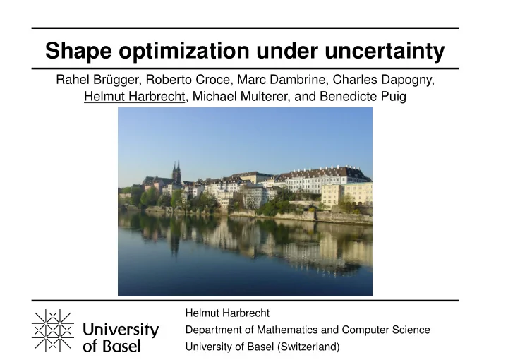
Shape optimization under uncertainty Rahel Br ugger, Roberto Croce, - - PowerPoint PPT Presentation

Shape optimization under uncertainty

Rahel Br¨ ugger, Roberto Croce, Marc Dambrine, Charles Dapogny, Helmut Harbrecht, Michael Multerer, and Benedicte Puig

Helmut Harbrecht Department of Mathematics and Computer Science University of Basel (Switzerland)

Overview

I Shape optimization in case of geometric uncertainty I Shape optimization in case of random diffusion I Shape optimization in case of random right-hand sides

Helmut Harbrecht

Free boundary problems

• Problem. Seek the free boundary Γ such that u satisfies

∆u = f

in D

u = g

• n Σ

u = 0, ∂u ∂n = h on Γ Σ D Γ I Growth of anodes. f ⌘ 0, g ⌘ 1, h ⌘ const Bernoulli’s free boundary problem I Electromagnetic shaping. Exterior boundary value

problem, uniqueness ensured by volume constraint. Different formulations as shape optimization problem.

J1(D) =

Z

D

• k∇vk2 2fv+h2

dx ! inf J2(D) =

Z

Dk∇(vw)k2dx ! inf

J3(D) =

Z

Γ

✓∂v ∂n +h ◆2 dx ! inf J4(D) =

Z

Γw2dx ! inf

9 > > > > > > > > > = > > > > > > > > > ;

where

8 > > < > > : ∆v = f ∆w = f

in D

v = g w = g

• n Σ

v = 0 ∂w ∂n = h

• n Γ

Helmut Harbrecht

Free boundary problems

• Problem. Seek the free boundary Γ such that u satisfies

∆u = f

in D

u = g

• n Σ

u = 0, ∂u ∂n = h on Γ Σ D Γ I Growth of anodes. f ⌘ 0, g ⌘ 1, h ⌘ const Bernoulli’s free boundary problem I Electromagnetic shaping. Exterior boundary value

problem, uniqueness ensured by volume constraint. Different formulations as shape optimization problem.

J1(D) =

Z

D

• k∇vk2 2fv+h2

dx ! inf J2(D) =

Z

Dk∇(vw)k2dx ! inf

J3(D) =

Z

Γ

✓∂v ∂n +h ◆2 dx ! inf J4(D) =

Z

Γw2dx ! inf

9 > > > > > > > > > = > > > > > > > > > ;

where

8 > > < > > : ∆v = f ∆w = f

in D

v = g w = g

• n Σ

v = 0 ∂w ∂n = h

• n Γ

Helmut Harbrecht

Free boundary problem with geometric uncertainty

• Problem. Seek the free boundary Γ(ω) such that u(ω) satisfies

∆u(ω) = 0

in D(ω)

u(ω) = 1

• n Σ(ω)

u(ω) = 0, ∂u ∂n(ω) = h on Γ(ω) Σ D Γ

for all ω 2 Ω. The questions to be addressed in the following are

I How to model the random domain D(ω)? Is the problem well-posed in the sense of D(ω) being almost surely well-defined? I Since it is a free boundary problem, we are looking for a free boundary. I Indeed, we are looking for the statistics of the domain itself. But how to define the

expectation of a random domain?

I How to compute the solution to the random free boundary problem numerically?

Helmut Harbrecht

Statistical quantities

I Expectation or mean. E[v](x) :=

Z

Ωv(x,ω)dP(ω)

I Correlation. Cor[v](x,y) :=

Z

Ωv(x,ω)v(y,ω)dP(ω) = E[v(x)v(y)]

I Covariance. Cov[v](x,y) :=

Z

Ω

• v(x,ω)E[v](x)
• v(y,ω)E[v](y)
• dP(ω)

= Cor[v](x,y)E[v](x)E[v](y) I Variance. V[v](x) :=

Z

Ω

• v(x,ω)E[v](x)

2dP(ω) = Cor[v](x,y)

• x=y E[v]2(x) = Cov[v](x,y)
• x=y

I k-th moment.

M [v](x1,x2,...,xk) :=

Z

Ωv(x1,ω)v(x2,ω)···v(xk,ω)dP(ω)

Helmut Harbrecht

Existence and uniqueness of solutions

Remarks.

I The solution Γ to the free boundary problem exists if h > 0 is sufficiently large. I If the interior boundary Σ is convex, then the solution is unique. I If the interior boundary Σ is not convex, multiple solutions might exist. I In case of a starshaped boundary Σ, the solution is unique and also starshaped.

• Parametrization. Assume that Σ(ω) is P-almost surely starlike. Then, we can parametrize

Σ(ω) =

• x = σ(φ,ω) 2 R2 : σ(φ,ω) = q(φ,ω)er(φ), φ 2 [0,2π]

, Γ(ω) =

• x = γ(φ,ω) 2 R2 : γ(φ,ω) = r(φ,ω)er(φ), φ 2 [0,2π]

.

Theorem (H/Peters [2015]). Assume that q(φ,ω) satisfies

0 < r  q(φ,ω)  R

for all φ 2 [0,2π] and P-almost every ω 2 Ω. Then, there exists a unique free boundary Γ(ω), for almost every ω 2 Ω. Espe- cially, with some constant R > R, the radial function r(φ,ω) of the associated free boundary satisfies

q(φ,ω) < r(φ,ω)  R

for all φ 2 [0,2π] and P-almost every ω 2 Ω.

Helmut Harbrecht

Expectation and variance

Definition (Parametrization based expectation). The parametrization based ex- pectation EP[D] of the boundaries Σ(ω) and Γ(ω) is given by

EP[Σ] =

• x 2 R2 : x = E[q(φ,·)]er(φ), φ 2 [0,2π]

, EP[Γ] =

• x 2 R2 : x = E[r(φ,·)]er(φ), φ 2 [0,2π]

.

• Remark. The expected domain EP[D] is thus given by

EP[D] =

• x = (ρ,φ) 2 R2 : E[q(φ,·)]  ρ  E[r(φ,·)]

.

This is also called the radius-vector expectation. Theorem (H/Peters [2015]). The variance of the domain D(ω) in the radial direction is given via the variances of its boundaries parameterizations in accordance with

VP[Σ(ω)] =

• x 2 R2 : x = V[q(φ,·)]er(φ), φ 2 [0,2π]

, VP[Γ(ω)] =

• x 2 R2 : x = V[r(φ,·)]er(φ), φ 2 [0,2π]

. The parametrization based expectation depends on the particular parametrization!

Helmut Harbrecht

Stochastic quadrature method

I Random parametrization of the interior boundary. q(φ,y) = E[q](φ)+

N

∑

k=1

qk(φ)yk

for y = [y1,...,yN]| 2 ⇤ := [1/2,1/2]N. It then holds

E[q](φ) =

Z

Ωq(φ,ω)dP(ω) =

Z

⇤q(φ,y)ρ(y)dy,

V[q](φ) =

Z

Ω

• q(φ,ω)

2dP(ω)

• E[q](φ)

2 =

Z

⇤

• q(φ,y)

2ρ(y)dy

• E[q](φ)

2. I Solution map. Let F : L∞ Ω;Cper(0,2π)

• ! L∞

Ω;Cper(0,2π)

• , q(φ,ω) 7! r(φ,ω)

denote the solution map. Then, the expectation and the variance of r(φ,ω) are given by

E[r](φ) = E[F(q)](φ)

and

V[r](φ) = V[F(q)](φ). I (Quasi-) Monte Carlo quadrature. The high-dimensional integrals are approximated

by means of a sampling method.

Helmut Harbrecht

Numerical example

q(φ,ω) = q(φ,ω)+

10

∑

k=1

p 2 k

• sin(kφ)Y2k1(ω)+cos(kφ)Y2k(ω)

1 2 3 4 5 6 0.05 0.1 0.15 0.2 0.25 0.3 0.35 0.4

Polar angle Radius

E[r] F (E[q]) E[q] std[r]

Helmut Harbrecht

Vorob’ev expectation

I Leading idea. Identify the random set D(ω) with its characteristic function 1D(ω)(x) = ( 1,

if x 2 D(ω),

0,

• therwise.

This embeds the problem into the linear space L∞(R2).

I Coverage function. The average of characteristic func-

tions is not a characteristic function anymore but belongs to the cone {q 2 L∞(R2) : 0  q  1}. The limit object is the so-called coverage function

p(x) = P

• x 2 D(ω)
• .

Definition (Vorob’ev expectation). The Vorob’ev expectation EV [D] of D(ω) is defined as the set {x 2 R2 : p(x) µ} for µ 2 [0,1] which is determined from the condition

L({x 2 R2 : p(x) λ}) 

Z

R2 p(x)dx  L({x 2 R2 : p(x) µ})

for all λ > µ.

Helmut Harbrecht

Numerical example

Helmut Harbrecht

Free boundary problem with random diffusion

• Problem. Seek the free boundary Γ(ω) such that u(ω) satisfies

div

• α(ω)∇u(ω)
• = 0

in D(ω)

u(ω) = 1

• n Σ

u(ω) = 0, α(ω)∂u ∂n(ω) = h on Γ(ω) Σ D Γ

for all ω 2 Ω, where

0 < α  α(ω)  α < ∞.

Theorem (Br¨ ugger/Croce/H [2018]). For ω 2 Ω, the solution

• u(ω),Γ(ω)
• is given by the shape optimization problem

J(D,ω) =

Z

D

⇢ α(ω)k∇u(ω)k2 + h2 α(ω)

• dx ! inf

subject to

div

• α(ω)∇u(ω)
• = 0 in D

u(ω) = 1 on Σ u(ω) = 0 on Γ

Helmut Harbrecht

Free boundary problem with random diffusion

I We shall minimize E ⇥ J(D,ω) ⇤ =

Z

D

Z

Ω

⇢ α(ω)k∇u(ω)k2 + h2 α(ω)

• dP(ω)dx ! min.

I A minimizer exists since we have an energy type shape functional. I The shape gradient reads δE ⇥ J(D,ω) ⇤ [V] =

Z

ΓhV,ni

Z

Ω

⇢ α(ω)k∇u(ω)k2 + h2 α(ω)

• dP(ω)dσ.

I Compute the Karhunen-Lo`

eve expansion of the diffusion coefficient

α(x,ω) = E[α](x)+

M

∑

k=1

αk(x)Yk(ω),

where the coefficient functions {αk(x)}k are elements of C1(D) and the random vari- ables {Yk(ω)}k are independently and uniformly distributed in [1/2,1/2]

yields a parametric problem on ⇤ = [1/2,1/2]M I Use a quasi Monte-Carlo method to approximate the integral over Ω by an integral over

• ver ⇤.

Helmut Harbrecht

Numerical results

random diffusion with E[α] = 1 and Cov[α](x,x0) = 0.2exp(kxx0k2)

• 1.5
• 1
• 0.5

0.5 1 1.5

• 1.5
• 1
• 0.5

0.5 1 1.5

h = 1

• 1
• 0.5

0.5 1

• 1
• 0.5

0.5 1

h = 3

• 1
• 0.5

0.5 1

• 1
• 0.5

0.5 1

h = 5

deterministic diffusion (α = 1)

• 1.5
• 1
• 0.5

0.5 1 1.5

• 1.5
• 1
• 0.5

0.5 1 1.5

h = 1

• 1
• 0.5

0.5 1

• 1
• 0.5

0.5 1

h = 3

• 1
• 0.5

0.5 1

• 1
• 0.5

0.5 1

h = 5

Helmut Harbrecht

Numerical results

random diffusion with E[α] = 1 and Cov[α](x,x0) = 0.15exp(kxx0k2)

• 2
• 1.5
• 1
• 0.5

0.5 1 1.5 2

• 1.5
• 1
• 0.5

0.5 1 1.5

h = 1

• 1.5
• 1
• 0.5

0.5 1 1.5

• 1
• 0.5

0.5 1

h = 2

• 1.5
• 1
• 0.5

0.5 1 1.5

• 1
• 0.5

0.5 1

h = 3

deterministic diffusion (α = 1)

• 2
• 1.5
• 1
• 0.5

0.5 1 1.5 2

• 1.5
• 1
• 0.5

0.5 1 1.5

h = 1

• 1.5
• 1
• 0.5

0.5 1 1.5

• 1
• 0.5

0.5 1

h = 2

• 1.5
• 1
• 0.5

0.5 1 1.5

• 1
• 0.5

0.5 1

h = 3

Helmut Harbrecht

Shape optimization for random right-hand sides

I Consider an elliptic state equation with random right-hand side, for example, the equa-

tions of linear elasticity with random forcing:

div ⇥ Ae

• u(ω)

⇤ = f(ω)

in D,

Ae

• u(ω)
• n = 0
• n Γfree

N ,

Ae

• u(ω)
• n = g(ω)
• n Γfix

N ,

u = 0

• n ΓD.

where e(u) = (∇u+∇uT)/2 stands for the linearized strain tensor and A is given by

AB = 2µB+λtr(B)I for all B 2 Rd⇥d

with the Lam´ e coefficients λ and µ satisfying µ > 0 and λ+2µ/d > 0.

I Consider a quadratic shape functional, for example, the compliance of shapes:

C(D,ω) =

Z

DAe

• u(x,ω)
• : e
• u(x,ω)
• dx

=

Z

Dhf(ω),u(ω)idx+

Z

Γfix

N

hg(x,ω),u(x,ω)idσx, I We aim at minimizing the expectation E[C(D,ω)] of the quadratic shape functional.

Helmut Harbrecht

PDEs with random right-hand side

Random boundary value problem:

div ⇥ α∇u(ω) ⇤ = f(ω) in D, u(ω) = 0 on ∂D

• ! the random solution depends linearly on the random input parameter

Theorem (Schwab/Todor [2003]): It holds

div ⇥ α∇E[u] ⇤ = E[f] in D, E[u] = E[g] on ∂D

and

(div⌦div) ⇥ (α⌦α)(∇⌦∇)Cor[u] ⇤ = Cor[f]

in D⇥D,

Cor[u] = 0

• n ∂(D⇥D).

Numerical solution of the correlation equation:

I sparse grid approximation by the combination technique

• H. Harbrecht, M. Peters, and M. Siebenmorgen. Combination technique based k-th moment analysis of elliptic

problems with random diffusion. J. Comput. Phys., 252:128–141, 2013.

I low-rank approximation by the pivoted Cholesky decomposition

• H. Harbrecht, M. Peters, and R. Schneider. On the low-rank approximation by the pivoted Cholesky decomposition.
• Appl. Numer. Math., 62:428–440, 2012.

I adaptive low-rank approximation by means of H -matrices

• J. D¨
• lz, H. Harbrecht, and C. Schwab. Covariance regularity and H -matrix approximation for rough random fields.
• Numer. Math., 135(4):1045–1071, 2017.

Helmut Harbrecht

Deterministic reformulation of the shape functional

Theorem (Dambrine/Dapogny/H [2015]). The expectation of the quadratic shape functional can be rewritten by

E[C(D,ω)] =

Z

D

• (Aex : ey)Cor[u]
• (x,y)
• x=y dx,

where

(Aex : ey) : ⇥ H1

ΓD(D)

⇤d ⌦ ⇥ H1

ΓD(D)

⇤d ! L2(D)⌦L2(D)

is the linear operator induced from the bilinear mapping

uvT 7! Ae(u) : e(v).

• Proof. The assertion follows from

E[C(D,ω)] =

Z

Ω

Z

DAe

• u(x,ω)
• : e
• u(x,ω)
• dx

=

Z

D

 (Aex : ey)

Z

Ωu(x,ω)u(y,ω)TdP(ω)

• x=y

dx =

Z

D

• (Aex : ey)Cor[u]
• (x,y)
• x=ydx.

⇤

Helmut Harbrecht

How to compute the correlation?

Theorem (Dambrine/Dapogny/H [2015]). The two-point correlation function

Cor[u] 2 [H1

ΓD(D)]d ⌦[H1 ΓD(D)]d

is the unique solution to the following tensor-product boundary value problem:

(divx⌦divy) ⇥ (Aex ⌦Aey)Cor[u] ⇤ = Cor[f]

in D⇥D,

(divx⌦Iy)(Aex ⌦Aey)Cor[u](Ix ⌦ny) = 0

• n D⇥Γfix[free

N

, (Ix ⌦divy)(Aex ⌦Aey)Cor[u](nx ⌦Iy) = 0

• n Γfix[free

N

⇥D, (divx⌦Iy)(Aex ⌦Iy)Cor[u] = 0

• n D⇥ΓD,

(Ix ⌦divy)(Ix ⌦Aey)Cor[u] = 0

• n ΓD ⇥D,

(Aex ⌦Aey)Cor[u](nx ⌦ny) = 0

• n
• Γfix[free

N

⇥Γfix[free

N

• \(Γfix

N ⇥Γfix N ),

(Aex ⌦Aey)Cor[u](nx ⌦ny) = Cor[g]

• n Γfix

N ⇥Γfix N ,

(Aex ⌦Iy)Cor[u](nx ⌦Iy) = 0

• n Γfix[free

N

⇥ΓD, (Ix ⌦Aey)Cor[u](Ix ⌦ny) = 0

• n ΓD ⇥Γfix[free

N

, Cor[u] = 0

• n ΓD ⇥ΓD.
• Proof. The assertion follows by tensorizing the state equation and the exploiting the linear-

ity when taking the expectation.

⇤

Helmut Harbrecht

Computing the shape gradient

Theorem (Dambrine/Dapogny/H [2015]). The functional E[J(D,ω)] is shape dif- ferentiable at any shape D 2 Uad and its derivative reads

δE ⇥C(D,ω) ⇤ [V] =

Z

Γfree

N

hV,ni

• (Aex : ey)Cor[u]
• (x,y)
• x=ydσx.
• Proof. The assertion follows from

δE ⇥C(D,ω) ⇤ [V] = E ⇥ δC(D,ω)[V] ⇤ =

Z

Ω

Z

Γfree

N

hV,ni

• Ae
• u(x,ω)
• : e
• u(x,ω)
• dσx

=

Z

Γfree

N

hV,ni  (Aex : ey)

Z

Ωu(x,ω)u(y,ω)TdP(ω)

• x=y

dσx =

Z

Γfree

N

hV,ni

• (Aex : ey)Cor[u]
• (x,y)
• x=ydσx.

⇤

Helmut Harbrecht

Low-rank approximation

I Approximation of the input correlation. Assume low-rank approximations Cor[f] ⇡ ∑

i

fifT

i ,

Cor[g] ⇡ ∑

j

g jgT

j.

Such expansions can efficiently be computed by e.g. a pivoted Cholesky decomposition.

I Approximation of the shape functional. The shape functional is simply given by E[C(D,ω)] =

Z

D∑ i, j

Ae(ui,j) : e(ui,j)dx,

where

div ⇥ Ae(ui,j) ⇤ = fi

in D,

Ae(ui, j)n = 0

• n Γfree

N ,

Ae(ui, j)n = g j

• n Γfix

N ,

ui,j = 0

• n ΓD.

I Approximation of the shape gradient. The shape gradient is given by δE ⇥C(D,ω) ⇤ [V] =

Z

Γfree

N

hV,ni∑

i,j

Ae(ui,j) : e(ui, j)dσx. I Alternative approach. A direct discretization of Cor[u] in a sparse grid space is possible

as well.

Helmut Harbrecht

First example

• Problem. A bridge is clamped on its lower part two sets of

loads ga = (1,1) and gb = (1,1) are applied on its top, i.e.,

g(x,ω) = ξ1(ω)ga(x)+ξ2(ω)gb(x).

The choice E[ξi] = 0, V[ξi] = 1, Cor[ξ1,ξ2] = α implies

Cor[g] = gagT

a +gbgT b +α

⇣ gagT

b +gbgT a

⌘ .

Sketch:

ΓN ΓD 1 1 ga gb

Convergence histories for the mean value and the volume:

10 20 30 40 50 60 70 80 90 50 100 150 200 250 alpha = -1 alpha = -0.7 alpha = 0 alpha = 0.5 alpha = 0.8 alpha = 1 0.3 0.4 0.5 0.6 0.7 0.8 0.9 1 50 100 150 200 250 alpha = -1 alpha = -0.7 alpha = 0 alpha = 0.5 alpha = 0.8 alpha = 1

Initial guess:

Helmut Harbrecht

First example

α = 1 α = 0.7 α = 0 α = 0.5 α = 0.8 α = 1

Helmut Harbrecht

Second example

• Problem. A bridge is clamped on its lower part two sets of loads gi =

(gi

1,gi 2), i = 1,2,3, are applied on its top such that

Cor[gi

1](x,y) = 105h+ i

✓x1 +y1 2 ◆ e10|x1y1|, Cor[gi

2](x,y) = 106k+ i

✓x1 +y1 2 ◆ e10|x1y1|,

where

h1(t) = 14 ✓ t 1 2 ◆2 , k1(t) = ( (4t 1)2,

if t  1

2,

(4t 3)2,

else,

h2(t) = 2t(1t)+ 1 2, k2(t) = ( (4t 1)(6t 2),

if t  1

2,

(4t 3)(6t 4),

else,

h3(t) = 1, k3(t) = ( 4t 1)(6t 1),

if t  1

2,

• 4t 3)(6t 5),

else.

Sketch:

ΓN ΓD 2 1

g

Initial guess:

Helmut Harbrecht

Second example

surface load g1(ω) surface load g2(ω) surface load g3(ω)

Helmut Harbrecht

About measurement noise in EIT

• Problem. Minimize

F(D) = (1α)E ⇥ J(D,ω) ⇤ +α q V ⇥ J(D,ω) ⇤ ! inf,

where the random shape functional reads as

J(D,ω) =

Z

D

• ∇
• v(ω)w
• 2dx ! inf

and the states read as

∆v(ω) = 0 ∆w = 0

in D,

v(ω) = 0 w = 0

• n Γ,

∂v ∂n(ω) = g(ω) w = f

• n Σ.

We assume that the Neumann data g are given as a Gaussian random field

g(x,ω) = g0(x)+

M

∑

i=1

gi(x)Yi(ω),

where the random variables are independent, satisfying Yi ⇠ N (0,1).

Helmut Harbrecht

Taking measurement noise in EIT into account

It holds for the shape functional

E ⇥ J(D,ω) ⇤ =

M

∑

i=1

Z

Σvigidσ+

Z

Σ

✓ g0 ∂w ∂n ◆ (v0 f)dσ, V ⇥ J(D,ω) ⇤ = 2

M

∑

i, j=1

✓Z

Σvig j dσ

◆2 +4

M

∑

i=1

✓Z

Σgi(v0 f)dσ

◆2

and for the shape gradient

δE ⇥ J(D,ω) ⇤ [V] =

Z

ΓhV,ni

" M

∑

i=0

✓∂vi ∂n ◆2

• ✓∂w

∂n ◆2# dσ, δV ⇥ J(D,ω) ⇤ [V] = 4

M

∑

i,j=1

✓Z

Σvigj dσ

◆✓Z

ΓhV,ni∂vi

∂n ∂v j ∂n dσ ◆ +8

M

∑

i=1

✓Z

Σgi(v0 f)dσ

◆✓Z

ΓhV,ni∂vi

∂n ∂v0 ∂n dσ ◆ .

where

∆vi = 0 in D, vi = 0 on Γ, ∂vi ∂n = gi on Σ.

Helmut Harbrecht

Numerical results (5% noise, 10 samples)

Reconstructions for different realizations of the measurement: Reconstructions for α = 0, α = 0.5, α = 0.75, α = 0.875

Helmut Harbrecht

Conclusion

I We considered several sources of uncertainty in shape optimization. I We discussed the notion of expected domains and introduced the para-

metrization based expectation as well as the Vorob’ev expectation. The computations require a huge number of solutions of the shape optimiza- tion problem under consideration.

I A free boundary problem with random diffusion has been treated by mini-

mizing a mean energy functional. This results in a high-dimensional state equation.

I Shape optimization of the expectation and/or the variance of a polynomial

shape functional and a state with random right-hand side is a deterministic

• problem. The mean of quadratic shape functionals can be even computed

without assuming a specific model for the randomness.

I Numerical results have been presented to illustrate the results.

Helmut Harbrecht

References

• R. Br¨

ugger, R. Croce, and H. Harbrecht. Solving a Bernoulli type free boundary problem with random diffusion. ESAIM Control Optim. Calc. Var., to appear.

• M. Dambrine, C. Dapogny, and H. Harbrecht.

Shape optimization for quadratic functionals and states with random right-hand sides. SIAM J. Control Optim., 53(5):3081–3103, 2015.

• M. Dambrine, H. Harbrecht, M. Peters, and B. Puig.

On Bernoulli’s free boundary problem with a random boundary.

• Int. J. Uncertain. Quantif., 7(4):335–353, 2017.
• M. Dambrine, H. Harbrecht, and B. Puig.

Incorporating knowledge on the measurement noise in electrical impedance tomography. ESAIM Control Optim. Calc. Var., to appear.

• H. Harbrecht and M. Peters.

Solution of free boundary problems in the presence of geometric uncertainties. Topological Optimization and Optimal Transport in the Applied Sciences, pp. 20–39, de Gruyter, 2017. Helmut Harbrecht