SHAPE ANALYSIS OF FUNCTIONAL DATA Anuj Srivastava Joint work with - PowerPoint PPT Presentation
SHAPE ANALYSIS OF FUNCTIONAL DATA Anuj Srivastava Joint work with Sutanoy Dasgupta, Ian Jermyn, Debdeep Pati Department of Statistics, Florida State University Presented at Statistical Modeling for Shapes and Imaging Workshop, IHP , Paris,
SHAPE ANALYSIS OF FUNCTIONAL DATA Anuj Srivastava Joint work with Sutanoy Dasgupta, Ian Jermyn, Debdeep Pati Department of Statistics, Florida State University Presented at Statistical Modeling for Shapes and Imaging Workshop, IHP , Paris, March 2019 Anuj Srivastava SHAPE ANALYSIS OF FUNCTIONAL DATA
Main Message Functional data analysis is fast growing topic area in statistics. Instead of using full functions in statistical models and analysis, there is a need to focus on their shapes. At the very least, one should separate shape and non-shape variables and treat them individually! Merging of tools from shape analysis and functional data analysis communities – traditionally two different sets of people – leads to a richer set of tools for automated data analysis.
Outline Introduction 1 Functional Data Analysis 2 Shape Analysis of Functional Data 3 Functional Regression Shape Modeling of Functional Data Shape-Constrained Function Estimation Probability Density Estimation 4 Unconstrained Density Estimation Shape-Constrained Density Estimation Summary 5 Anuj Srivastava SHAPE ANALYSIS OF FUNCTIONAL DATA
Statistical Shape Analysis Tremendous amount of research in this general area. Excellent partnerships between geometry, statistics, topology, graphics, image analysis, etc. A variety of objects of interest – curves in Euclidean spaces, surfaces, curves on manifolds, tree-like structures, etc. 0.4 0.2 0 −0.2 −0.4 −0.6 0.5 0 1 −0.5 0.5 0 curves surfaces trajectories tree-like structures Applications include computer vision, medical imaging, bioinformatics, and so on. These applications usually involve image data. Shape analysis has a much bigger role to play, in a much more general scenario. Not just imaging data.
Shape Analysis Tasks Shape Analysis: A set of theoretical and computational tools that can provide: Shape Metric: Quantify differences in any two given shapes. Shape Deformation/Geodesic: How to optimally deform one shape into another. Shape summary: Compute sample mean, sample covariance, PCA, and principal modes of shape variability. Shape model: Develop statistical models and perform hypothesis testing. Shape testing: ANOVA, two-sample test, k -sample test, etc.
Some Success Stories From our group, many more from other groups: Quantify effects of lifestyle (running and sedentary) on mitochondria morphology in mice. Shape estimation of 3D chromosomes from single cell Hi-C (human and mice embryonic stem cells). Change point detection in human functional brain connectivity using fMRI of subjects performing tasks. Structural changes in subcortical morphology due to cognitive disorders – ADHD, Alzheimers. Representation and classification of activities in Youtube videos by covariance trajectories of DNN features. Understanding changes in neuron morphology under gene knockouts. Analysis of kinect-based shape trajectories for physical therapy and evaluation.
Outline Introduction 1 Functional Data Analysis 2 Shape Analysis of Functional Data 3 Functional Regression Shape Modeling of Functional Data Shape-Constrained Function Estimation Probability Density Estimation 4 Unconstrained Density Estimation Shape-Constrained Density Estimation Summary 5 Anuj Srivastava SHAPE ANALYSIS OF FUNCTIONAL DATA
Functional Data Analysis (FDA) Functional Data Analysis: A term coined by Jim Ramsay and colleagues– perhaps in late 1980s or even earlier. Data analysis where random quantities of interest are functions, i.e. elements of a function space F . f : D → R or f : D → M . Statistical modeling and inference takes place on a function space. One typically needs a metric structure, often it is the L 2 Hilbert structure. Several textbooks have been written with their own strengths and weaknesses. One of the fastest growing area in statistics community. Where can one find functional data? Everywhere!
What are the Tasks in FDA? For the most part it is same as any statistics domain. Having chosen the metric structure on the function spaces, one can: Summarize functional data: central tendency in the data (mean, median), covariance, principal modes of variability. Inference on function spaces: Model the function observations, observation = signal + noise , followed by estimation theory, analysis. Test hypothesis involving observations of functional variables. This includes classification, clustering, two-sample test, ANOVA, etc. Regress, Predict: Develop regression models where functional variables are predictors, responses, or both!
Foundational Pillar of Current FDA The key item is the choice of a metric! Most of the FDA literature (statistics) is centered around the Hilbert structure induced by the L 2 norm. But there are some major problems with this choice. Distances (under L 2 metric) don’t always match with our intuition. d 12 = 0.837, d 13 = 0.791 d 12 = 4.471, d 13 = 3.989 1 14 f 1 f 1 f 2 12 f 2 f 3 f 3 0.5 10 8 0 6 4 -0.5 2 -1 0 0 0.2 0.4 0.6 0.8 1 0 0.2 0.4 0.6 0.8 1 In case functional data has phase or misalignment variability, it can completely throw off current FDA solutions.
Functional Statistics with Phase Variability Recall that the average under L 2 norm is given by: n f ( t ) = 1 ¯ � f i ( t ) . n i = 1 Function averages under the L 2 norm are not representative! 8 8 7 6 6 5 4 4 2 3 2 0 1 0 -2 -1 -0.5 0 0.5 1 -1 -0.5 0 0.5 1 { f i } , ¯ ¯ f f ± std Individual functions are all bimodal and the average is multimodal! In ¯ f , the geometric features (peaks and valleys) are smoothed out. (They are interpretable attributes in many situations and they need to be preserved.)
FPCA With Phase Variability n = 50 functions, f i ( t ) = f 0 ( γ i ( t )) , γ i s are random time warps. 4 4 70 3.5 3.5 60 3 3 50 2.5 2.5 40 2 2 30 1.5 1.5 20 1 1 10 0.5 0.5 0 0 0 0 0.2 0.4 0.6 0.8 1 0 0.2 0.4 0.6 0.8 1 0 10 20 30 40 50 function data { f i } mean ˆ µ f singular values 4 4 3 3.5 2.5 3 3 2 2.5 2 2 1.5 1 1.5 1 1 0 0.5 0.5 -1 0 0 0 0.2 0.4 0.6 0.8 1 0 0.2 0.4 0.6 0.8 1 0 0.2 0.4 0.6 0.8 1 µ ± σ 1 U 1 µ ± σ 2 U 2 µ ± σ 3 U 3 Principal components seem to show vertical variability even though the data is completely horizontal.
FPCA: Data With Phase Variability 10 5 component 2 component 3 5 0 0 5 -5 -5 0 -10 0 10 20 -5 0 5 10 -5 0 5 10 component 1 component 1 10 5 10 component 1 component 3 5 0 5 0 -5 -5 0 -10 0 10 -10 0 10 -5 0 5 component 2 component 2 6 10 5 component 1 component 2 5 4 0 0 2 -5 -5 0 -10 0 10 -10 0 10 -5 0 5 component 3 component 3
Real Issue L 2 norm uses vertical registration: � 1 � f 1 − f 2 � 2 = ( f 1 ( t ) − f 2 ( t )) 2 dt . 0 For each t , f 1 ( t ) is being compared with f 2 ( t ) . 2 2 1 1.5 1.5 1 1 0.5 0.5 0.5 0 0 0 -0.5 -0.5 -1 -1 -0.5 -1.5 -1.5 -2 -2 -1 0 0.2 0.4 0.6 0.8 1 0 0.2 0.4 0.6 0.8 1 0 0.2 0.4 0.6 0.8 1 In shape analysis of functions, a combination of vertical and horizontal variability is often more natural: 2 2 1.5 1.5 1 1 0.5 0.5 0 0 -0.5 -0.5 -1 -1 -1.5 -1.5 -2 -2 0 0.2 0.4 0.6 0.8 1 0 0.2 0.4 0.6 0.8 1 Registration Geodesic The question is: How can we detect and decompose difference into horizontal and vertical components? We need shape analysis of functional data!
Outline Introduction 1 Functional Data Analysis 2 Shape Analysis of Functional Data 3 Functional Regression Shape Modeling of Functional Data Shape-Constrained Function Estimation Probability Density Estimation 4 Unconstrained Density Estimation Shape-Constrained Density Estimation Summary 5 Anuj Srivastava SHAPE ANALYSIS OF FUNCTIONAL DATA
Notion of Shape for Functions Functions typically differ in: Number of modes Heights at modes and antimodes The placements (locations) of these modes. 3.5 3.5 3 3 2.5 2.5 2 2 1.5 1.5 1 1 0.5 0.5 0 0 0 0.2 0.4 0.6 0.8 1 0 0.2 0.4 0.6 0.8 1 Notion 1: Shape = modes Notion 2: Shape = modes + heights The desired notion of shape depends on the applications. Sometimes, Shape relates to number of modes . Or Shape relates to number of modes and their heights Can be even more specific – involving curvatures at the modes. However, the location is mostly left out as a nuisance variable, i.e. it does not affect the shape. To study shapes, the key idea is to separate placement (phase) variability from the shape variability.
Modeling Phase Variability The horizontal variability is controlled by actions of the diffeomorphism group Γ on function space: F = { f : D → R } . Shape classes are orbits under these actions. Several actions are possible: Height and Mode-Preserving : F × Γ → F , ( f , γ ) = f ◦ γ 1 5 4 0.8 3 0.6 2 0.4 1 0.2 0 -1 0 0 0.2 0.4 0.6 0.8 1 0 0.2 0.4 0.6 0.8 1 { γ i } { f ◦ γ i } The number and heights of modes are preserved. Area and norm are not preserved.
Diffeomorphism Group Actions Area-Preserving F × Γ → F , ( f , γ ) = ( f ◦ γ ) J γ where J γ is the determinant of the Jacobian of γ . 1 6 5 0.8 4 3 0.6 2 0.4 1 0 0.2 -1 0 -2 0 0.2 0.4 0.6 0.8 1 0 0.2 0.4 0.6 0.8 1 { γ i } { ( f ◦ γ i ) J γ i } � � ( f ◦ γ ) J γ dx . However, the modes and the norm Here we have fdx = of f can change.
Recommend
More recommend
Explore More Topics
Stay informed with curated content and fresh updates.
