Session 10: Fitting models: Central tendency and dispersion Stats - PowerPoint PPT Presentation
Session 10: Fitting models: Central tendency and dispersion Stats 60/Psych 10 Ismael Lemhadri Summer 2020 This time Building models to describe data Central tendency Dispersion and variability What is a model? Models simplify
Session 10: Fitting models: Central tendency and dispersion Stats 60/Psych 10 Ismael Lemhadri Summer 2020
This time • Building models to describe data • Central tendency • Dispersion and variability
What is a “model”?
Models simplify the world for us
The basic statistical model outcome = model + error what we difference what we actually between expected expect to observe and observed observe (the data) (our prediction) The model is should be much simpler than the thing it is modeling!
A simple example • What is the height of children in the NHANES sample?
NHANES <- NHANES %>% mutate(isChild = Age<18) NHANES_child <- NHANES %>% subset(subset=isChild & Height!='NA') ggplot(data=NHANES_child,aes(Height)) + geom_histogram(bins=100)
What is the simplest model we can image? • One guess: what about the most common value in the dataset (the mode )? • height(i) = 166.5 + error(i) • Summarizes 2,223 data points in terms of a single number • How well does that describe the data? • Computing the error: • error = outcome - model
error <- NHANES_child$Height - 166.5 ggplot(NULL,aes(error)) + geom_histogram(bins=100) average error: -27.94 inches
A better model? n • We would like for our ( x i − ¯ X error = X ) = 0 model to have zero error, i =1 on average n n • If we use the mean of the X X ¯ x i − X = 0 data as our model, then that will be the case i =1 i =1 n n P n X X ¯ x i = X i =1 x i ¯ X = i =1 i =1 n n X x i = n ¯ X i =1 n n X X x i = x i i =1 i =1
Sum of errors from the mean is zero d <- c(3,5,6,7,9) x error mean(d) 3 -3 ## [1] 6 5 -1 errors=d-mean(d) print(errors) 6 0 ## [1] -3 -1 0 1 3 7 1 print(sum(errors)) 9 3 ## [1] 0 sum=0
error_mean <- NHANES_child$Height - mean(NHANES_child$Height) ggplot(NULL,aes(error_mean)) + geom_histogram(bins=100) + xlim(-60,60) average error: -0.000000 inches
Building an even better model • The average error for mean is zero • But there are still errors, sometimes positive and sometimes negative • The “best” estimate is one that minimizes errors overall (both positive and negative) • We can quantify the total error by squaring the errors and adding them up n X x ) 2 sum of squared errors = ( x i − ˆ i =1 P n i =1 x i model prediction : ˆ x = mean ( x ) = n
We take the mean of the squared errors by dividing SSE by the number of values, and then take the square root: mean squared error = SSE N print(paste(‘average squared error:',mean(error_mean**2))) mean squared error: 720.05 This tells us that while on average we make no error, for any individual we could actually make quite a big error (~27 inches 2 on average). Could we make the model any better? What else do we know about these individuals that might help us better estimate their height?
What about their age? Let’s plot height versus age and see how they are related. ggplot(NHANES_child,aes(x=Age,y=Height)) + geom_point(position=‘jitter’) + geom_smooth()
# find the best fitting model to predict height given age model_age <- lm(Height ~ Age, data = NHANES_child) # the predict() function uses the fitted model to predict values for each person predicted_age <- predict(model_age) error_age <- NHANES_child$Height - predicted_age sprintf('average squared error: %f inches',mean(error_age**2)) mean squared error: 69.61 inches
What else do we know? • What other variables might be related to height?
ggplot(NHANES_child,aes(x=Age,y=Height)) + geom_point(aes(colour = factor(Gender)),position = "jitter",alpha=0.2) + geom_smooth(aes(group=factor(Gender),colour = factor(Gender)))
model_age_gender <- lm(Height ~ Age + Gender, data=NHANES_child) predicted_age_gender <- predict(model_age_gender) error_age_gender <- NHANES_child$Height - predicted_age_gender mean squared error: 66.42 inches model: height = 84.33 + 5.47*Age + 3.57*Gender
error_df <- data.frame(error=c(mean(error**2),mean(error_mean**2), mean(error_age**2),mean(error_age_gender**2))) row.names(error_df) <- c(‘mode','mean','age','age+gender') error_df$RMSE <- sqrt(error_df$error) ggplot(error_df,aes(x=row.names(error_df),y=RMSE)) + geom_col() +ylab('root mean squared error') + xlab('Model') + scale_x_discrete(limits = c('mode','mean','age','age+gender'))
What makes a model “good”? • Describes our dataset well • the error for the fitted data is low • Generalizes to other data • the error for a new dataset is low • These two are often in conflict!
Sources of error: • Remember the basic model: • outcome = model + error • Error can come from two sources: • The model is incorrect • The measurements have random error (“noise”)
low error: Error can come model is correct from two sources: noise is low • incorrect model • noisy data High error: High error: model is correct model is wrong noise is high noise is low
Original sample Overfitting SSE=4369 SSE=1026 • A more complex model will always fit the data better • The model fits the underlying signal as well as the random New sample noise in the data SSE=10615 • A simpler model often SSE=18505 does a better job of explaining a new sample from the same group
The principle of parsimony • “It can scarcely be denied that the supreme goal of all theory is to make the irreducible basic elements as simple and as few as possible without having to surrender the adequate representation of a single datum of experience.” • Albert Einstein, 1933 • Paraphrased as “everything should be as simple as it can be, but not simpler”
The simplest model: Central tendency • What is the most typical value?
Mean (aka average) sample mean population mean P n P n i =1 x i i =1 x i ¯ X = µ = N n same formula, different symbols
The mean as a balancing point
The mean is the “best” estimate • The mean is the value that minimizes the sum of squared errors • This is the statistical definition of being the “best” estimate • We proved this earlier • But we can also demonstrate it using R, which you will do in your next problem set… n X x ) 2 SSE = ( x i − ˆ i =1
Estimating the mean accurately can require lots of data Data: Height of children • from NHANES (2,223 children) Mean height: 138.5 in • What happens if we • take smaller samples from this group? start with a sample • of size 10 and then increase by 10 up to 1000
One not-so-useful feature of the mean people income people income Joe 48000 48000 Joe Karen 64000 Karen 64000 Mark 58000 Mark 58000 Andrea 72000 Andrea 72000 Beyonce 54,000,000 Pat 66000 mean income: $61,600 mean income: $10,848,400
Breakouts! • Come up with an example of a statistic that is relevant to public policy and that might be contaminated by outliers • What effect could this have on policy decisions? • How might you address the problem?
Median • When the scores are ordered from smallest to largest, the median is the middle score original: 8 6 3 14 12 7 6 4 9 sorted: 3 4 6 6 7 8 9 12 14 { { median = 7
Median • When the scores are ordered from smallest to largest, the median is the middle score • When there is an even number of scores, the median is the average between the middle two scores original: 8 6 3 14 12 7 6 4 9 13 sorted: 3 4 6 6 7 8 9 12 13 14 { { median = 7.5
Median as the 50th percentile original: 8 6 3 12 7 6 4 9 13
The median minimizes absolute error n • The mean minimizes the sum of X x ) 2 SSE = ( x i − ˆ squared errors i =1 n • The median minimizes the sum of X | x i − ˆ x | SAE = absolute errors i =1 Why do you think that matters?
The median is less sensitive to outliers people income people income Joe 48000 48000 Joe Karen 64000 Karen 64000 Mark 58000 Mark 58000 Andrea 72000 Andrea 72000 Beyonce 54,000,000 Pat 66000 mean income: $61,600 mean income: $10,848,400 median income: $64,000 median income: $64,000
Why would we ever use the mean instead of the median? • The mean is the “best” estimator • It bounces around less from sample to sample than any other estimator • More on this later • But the median is more robust • Less likely to be influenced by outliers • Statistics is all about tradeoffs…
Mode • What is the most common value in the dataset?
Bimodal distributions • There is not necessarily a single peak in the distribution Weaver worker ants “minor workers” “major workers” Minor worker grooming a major worker https://commons.wikimedia.org/wiki/File:BimodalAnts.png https://termitesandants.blogspot.com/2010/04/oecophylla-smaragdina.html
The fit of the sample mean: Variance and standard deviation i =1 ( x i − ¯ P n X ) 2 variance = SSE n − 1 = n − 1 √ SD = variance x error error^2 3 -3 9 SSE: 20 5 -1 1 6 0 0 variance (s 2 )=20/4=5 7 1 1 SD=sqrt(5)=2.2 9 3 9 mean=6
Recommend
More recommend
Explore More Topics
Stay informed with curated content and fresh updates.
