Selv-optimaliserende og eksplisitte metoder for online - PDF document
Selv-optimaliserende og eksplisitte metoder for online optimalisering Sigurd Skogestad Department of Chemical Engineering Norwegian University of Science and Tecnology (NTNU) Trondheim, Norway Effective Implementation of optimal operation
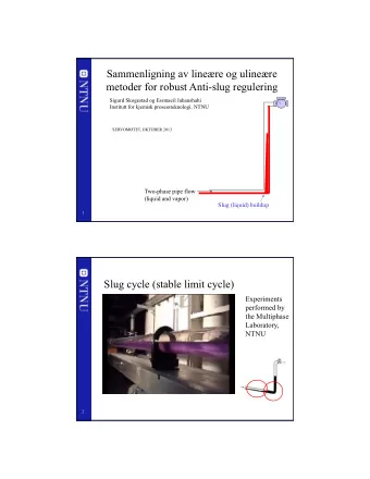
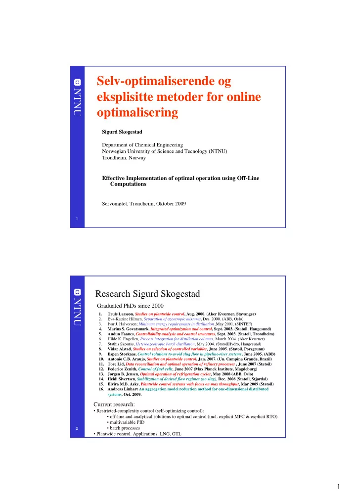
Selv-optimaliserende og eksplisitte metoder for online optimalisering Sigurd Skogestad Department of Chemical Engineering Norwegian University of Science and Tecnology (NTNU) Trondheim, Norway Effective Implementation of optimal operation using Off-Line Computations Servomøtet, Trondheim, Oktober 2009 1 Research Sigurd Skogestad Graduated PhDs since 2000 1. Truls Larsson, Studies on plantwide control , Aug. 2000. (Aker Kværner, Stavanger) 2. Eva-Katrine Hilmen, Separation of azeotropic mixtures , Des. 2000. (ABB, Oslo) 3. Ivar J. Halvorsen; Minimum energy requirements in distillation , May 2001. (SINTEF) 4. Marius S. Govatsmark, Integrated optimization and control , Sept. 2003. (Statoil, Haugesund) 5. Audun Faanes, Controllability analysis and control structures , Sept. 2003. (Statoil, Trondheim) 6. Hilde K. Engelien, Process integration for distillation columns , March 2004. (Aker Kværner) 7. Stathis Skouras, Heteroazeotropic batch distillation , May 2004. (StatoilHydro, Haugesund) 8. Vidar Alstad, Studies on selection of controlled variables , June 2005. (Statoil, Porsgrunn) Espen Storkaas, Control solutions to avoid slug flow in pipeline-riser systems , June 2005. (ABB) 9. 10. Antonio C.B. Araujo, Studies on plantwide control , Jan. 2007. (Un. Campina Grande, Brazil) 11. Tore Lid, Data reconciliation and optimal operation of refinery processes , June 2007 (Statoil) 12. Federico Zenith, Control of fuel cells, June 2007 (Max Planck Institute, Magdeburg) 13. Jørgen B. Jensen, Optimal operation of refrigeration cycles , May 2008 (ABB, Oslo) 14. Heidi Sivertsen, Stabilization of desired flow regimes (no slug) , Dec. 2008 (Statoil, Stjørdal) 15. Elvira M.B. Aske, P lantwide control systems with focus on max throughput , Mar 2009 (Statoil) 16. Andreas Linhart An aggregation model reduction method for one-dimensional distributed systems, Oct. 2009. Current research: • Restricted-complexity control (self-optimizing control): • off-line and analytical solutions to optimal control (incl. explicit MPC & explicit RTO) • multivariable PID • batch processes 2 • Plantwide control. Applications: LNG, GTL 1
Outline • Implementation of optimal operation • Paradigm 1: On-line optimizing control • Paradigm 2: "Self-optimizing" control schemes – Precomputed (off-line) solution • Examples • Control of optimal measurement combinations – Nullspace method – Exact local methom – Link to optimal control / Explicit MPC • Conclusion 3 Process control: Implementation of optimal operation RTO y 1s MPC y 2s PID u (valves) 4 2
Optimal operation • A typical dynamic optimization problem • Implementation: “Open-loop” solutions not robust to disturbances or model errors • Want to introduce feedback 5 Implementation of optimal operation • Paradigm 1: On-line optimizing control where measurements are used to update model and states • Paradigm 2: “ Self-optimizing” control scheme found by exploiting properties of the solution 6 3
Implementation: Paradigm 1 • Paradigm 1: Online optimizing control • Measurements are primarily used to update the model • The optimization problem is resolved online to compute new inputs. • Example: Conventional MPC • This is the “obvious” approach (for someone who does not know control) 7 Example paradigm 1: On-line optimizing control of Marathon runner • Even getting a reasonable model requires > 10 PhD’s … and the model has to be fitted to each individual…. • Clearly impractical! 9 4
Implementation: Paradigm 2 • Paradigm 2: Precomputed solutions based on off-line optimization • Find properties of the solution suited for simple and robust on-line implementation • Proposed method : Turn optimization into feedback problem. – Find regions of active constraints and in each region: 1. Control active constraints 2. Control “self-optimizing ” variables for the remaining unconstrained degrees of freedom • “inherent optimal operation” • Examples – Marathon runner – Hierarchical decomposition – Optimal control – Explicit MPC 10 Optimal operation - Runner Solution 2 – Feedback (Self-optimizing control) – What should we control? 11 5
Optimal operation - Runner Self-optimizing control: Sprinter (100m) • 1. Optimal operation of Sprinter, J=T – Active constraint control: • Maximum speed (”no thinking required”) 12 Optimal operation - Runner Self-optimizing control: Marathon (40 km) • Optimal operation of Marathon runner, J=T • Any self-optimizing variable c (to control at constant setpoint)? • c 1 = distance to leader of race • c 2 = speed • c 3 = heart rate • c 4 = level of lactate in muscles 13 6
Implementation paradigm 2: Feedback control of Marathon runner Simplest case: select one measurement c = heart rate measurements • Simple and robust implementation • Disturbances are indirectly handled by keeping a constant heart rate • May have infrequent adjustment of setpoint (heart rate) 14 Further examples self-optimizing control • Marathon runner • Central bank • Cake baking • Business systems (KPIs) • Investment portifolio • Biology • Chemical process plants Define optimal operation (J) and look for ”magic” variable (c) which when kept constant gives acceptable loss (self- optimizing control) 15 7
More on further examples • Central bank. J = welfare. u = interest rate. c=inflation rate (2.5%) • Cake baking. J = nice taste, u = heat input. c = Temperature (200C) • Business, J = profit. c = ”Key performance indicator (KPI), e.g. – Response time to order – Energy consumption pr. kg or unit – Number of employees – Research spending Optimal values obtained by ”benchmarking” • Investment (portofolio management). J = profit. c = Fraction of investment in shares (50%) • Biological systems: – ”Self-optimizing” controlled variables c have been found by natural selection – Need to do ”reverse engineering” : • Find the controlled variables used in nature • From this possibly identify what overall objective J the biological system has been attempting to optimize 16 Example paradigm 2: Optimal operation of chemical plant • Hierarchial decomposition based on time scale separation Self-optimizing control: Acceptable operation (=acceptable loss) achieved using constant set points (c s ) for the controlled variables c c s Controlled variables c 1. Active constraints 2. “Self-optimizing” variables c • for remaining unconstrained degrees of freedom (u) • No or infrequent online optimization. • Controlled variables c are found 17 based on off-line analysis. 8
Summary feedback approach: Turn optimization into setpoint tracking Issue: What should we control to achieve indirect optimal operation ? Primary controlled variables (CVs): 1. Control active constraints! 2. Unconstrained CVs: Look for “magic” self- optimizing variables! Need to identify CVs for each region of active constraints 18 “Magic” self-optimizing variables: How do we find them? • Intuition: “Dominant variables” (Shinnar) • Is there any systematic procedure? A. Senstive variables: “Max. gain rule” (Gain= Minimum singular value) B. “Brute force” loss evaluation C. Optimal linear combination of measurements, c = Hy 19 9
Unconstrained optimum Optimal operation Cost J J opt J opt c c opt opt Controlled variable c 20 Unconstrained optimum Optimal operation Cost J d J opt J opt n c opt c opt Controlled variable c Two problems: • 1. Optimum moves because of disturbances d: c opt (d) 21 • 2. Implementation error, c = c opt + n 10
Unconstrained optimum Candidate controlled variables c for self-optimizing control Intuitive 1. The optimal value of c should be insensitive to disturbances (avoid problem 1) 2. Optimum should be flat (avoid problem 2 – implementation error). Equivalently: Value of c should be sensitive to degrees of freedom u. • “Want large gain”, |G| • Or more generally: Maximize minimum singular value, Good Good BAD 22 Unconstrained optimum Quantitative steady-state: Maximum gain rule c u G Maximum gain rule (Skogestad and Postlethwaite, 1996): Look for variables that maximize the scaled gain (G s ) (minimum singular value of the appropriately scaled steady-state gain matrix G s from u to c) 23 11
Why is Large Gain Good? J, c Loss J opt G c opt c-c opt Variation of u u opt u With large gain G: Even large implementation error n in c translates into small deviation of u from u opt ( d ) - leading to lower loss 24 Unconstrained degrees of freedom: “Self-optimizing” variable combinations • Operational objective: Minimize cost function J(u,d) • The ideal “self-optimizing” variable is the gradient (first-order optimality condition (ref: Bonvin and coworkers)): • Optimal setpoint = 0 • BUT: Gradient can not be measured in practice • Possible approach: Estimate gradient J u based on measurements y • Here alternative approach: Find optimal linear measurement combination which when kept constant ( § n) minimize the effect of d on loss. Loss = J(u,d) – J(u opt ,d); where input u is used to keep c = constant § n • Candidate measurements (y): Include also inputs u 25 12
Recommend
More recommend
Explore More Topics
Stay informed with curated content and fresh updates.
