Optimal Control & Viscosity Solutions Tutorial Slides from - PowerPoint PPT Presentation

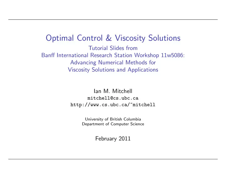
Optimal Control & Viscosity Solutions Tutorial Slides from Banff International Research Station Workshop 11w5086: Advancing Numerical Methods for Viscosity Solutions and Applications Ian M. Mitchell mitchell@cs.ubc.ca http://www.cs.ubc.ca/˜mitchell University of British Columbia Department of Computer Science February 2011

Outline ∙ Optimal control: models of system dynamics and objective functionals ∙ The value function and the dynamic programming principle ∙ A formal derivation of the Hamilton-Jacobi(-Bellman) equation ∙ Viscosity solutions and a rigorous derivation ∙ Other types of Hamilton-Jacobi equations in control ∙ Optimal control problems with analytic solutions ∙ References Optimal Control & Viscosity Solutions Ian M. Mitchell— UBC Computer Science 2/ 41

Control Theory ∙ Control theory is the mathematical study of methods to steer the evolution of a dynamic system to achieve desired goals ∙ For example, stability or tracking a reference ∙ Optimal control is a branch of control theory that seeks to steer the evolution so as to optimize a specific objective functional ∙ There are close connections with calculus of variations ∙ Mathematical study of control requires predictive models of the system evolution ∙ Assume Markovian models: everything relevant to future evolution of the system is captured in the current state ∙ Many classes of models, but we will talk primarily about deterministic, continuous state, continuous time systems ∙ Other continuous models: stochastic DEs, delay DEs, differential algebratic equations, differential inclusions, . . . ∙ Other classes of dynamic evolution: discrete time (eg: discrete event), discrete state (eg: Markov chains), . . . Optimal Control & Viscosity Solutions Ian M. Mitchell— UBC Computer Science 3/ 41

System Models ∙ Deterministic, continuous state, continuous time systems are often modeled with ordinary differential equations (ODEs) 푥 ( 푡 ) = 푑푥 ( 푡 ) ˙ = 푓 ( 푥 ( 푡 ) , 푢 ( 푡 )) 푑푡 with state 푥 ( 푡 ) ∈ ℝ 푑 푥 , input 푢 ∈ 풰 ⊆ ℝ 푑 푢 , and initial condition 푥 (0) = 푥 0 ∙ To ensure that trajectories are well-posed (they exist and are unique), it is typically assumed that 푓 is bounded and Lipschitz continuous with respect to 푥 for fixed 푢 ∙ The field of system identification studies how to determine 푓 ∙ An important subclass of system dynamics are linear 푥 ( 푡 ) = A 푥 + B 푢 ˙ with A ∈ ℝ 푑 푥 × 푑 푥 and B ∈ ℝ 푑 푥 × 푑 푢 ∙ Unless specifically described as “nonlinear control,” most engineering control theory (academic and practical) assumes linear systems Optimal Control & Viscosity Solutions Ian M. Mitchell— UBC Computer Science 4/ 41

Optimal Control Objectives ∙ Choose input signal 푢 ( ⋅ ) ∈ 픘 ≜ { 푢 : [0 , ∞ [ → 풰 ∣ 푢 ( ⋅ ) is measureable } to minimize the cost functional 퐽 ( 푥, 푢 ( ⋅ )) or 퐽 ( 푥, 푡, 푢 ( ⋅ )) ∙ Many possible cost functionals exist, such as: ∙ Finite horizon : given horizon 푇 > 0 , running cost ℓ and terminal cost 푔 ∫ 푇 퐽 ( 푥 ( 푡 ) , 푡, 푢 ( ⋅ )) ≜ ℓ ( 푥 ( 푠 ) , 푢 ( 푠 )) 푑푠 + 푔 ( 푥 ( 푇 )) 푡 ∙ Minimum time : given target set 풯 ⊂ ℝ 푑 푥 { min { 푡 ∣ 푥 ( 푡 ) ∈ 풯 } , if { 푡 ∣ 푥 ( 푡 ) ∈ 풯 } ∕ = ∅ ; 퐽 ( 푥 0 , 푢 ( ⋅ )) ≜ + ∞ , otherwise ∙ Discounted infinite horizon : given discount factor 휆 > 0 and running cost ℓ ∫ ∞ ℓ ( 푥 ( 푠 ) , 푢 ( 푠 )) 푒 − 휆푠 푑푠 퐽 ( 푥 0 , 푢 ( ⋅ )) ≜ 0 ∙ Alternatively, “maximize payoff functionals” or “optimize objective functionals” Optimal Control & Viscosity Solutions Ian M. Mitchell— UBC Computer Science 5/ 41

Outline ∙ Optimal control: models of system dynamics and objective functionals ∙ The value function and the dynamic programming principle ∙ A formal derivation of the Hamilton-Jacobi(-Bellman) equation ∙ Viscosity solutions and a rigorous derivation ∙ Other types of Hamilton-Jacobi equations in control ∙ Optimal control problems with analytic solutions ∙ References Optimal Control & Viscosity Solutions Ian M. Mitchell— UBC Computer Science 6/ 41

Value Functions ∙ The value function specifies the best possible value of the cost functional starting from each state (and possibly time) 푢 ( ⋅ ) ∈ 픘 퐽 ( 푥, 푢 ( ⋅ )) 푢 ( ⋅ ) ∈ 픘 퐽 ( 푥, 푡, 푢 ( ⋅ )) 푉 ( 푥 ) = inf or 푉 ( 푥, 푡 ) = inf ∙ Infimum may not be achievable ∙ If infimum is attained then the (possibly non-unique) optimal input is often designated 푢 ∗ ( ⋅ ) , and sometimes the corresponding optimal trajectory is designated 푥 ∗ ( ⋅ ) ∙ Intuitively, to find the best trajectory from a point 푥 , go to a neighbour ˆ 푥 of 푥 which minimizes the sum of the cost from 푥 to ˆ 푥 and the cost to go from ˆ 푥 . ∙ This intuition is formalized in the dynamic programming principle Optimal Control & Viscosity Solutions Ian M. Mitchell— UBC Computer Science 7/ 41

Dynamic Programming Principle ∙ For concreteness, we assume a finite horizon objective with horizon 푇 , running cost ℓ ( 푥, 푢 ) and terminal cost 푔 ( 푥 ) ∙ Dynamic Programming Principle (DPP): for each ℎ > 0 small enough that 푡 + ℎ < 푇 [∫ 푡 + ℎ ] 푉 ( 푥, 푡 ) = inf ℓ ( 푥 ( 푠 ) , 푢 ( 푠 )) 푑푠 + 푉 ( 푥 ( 푡 + ℎ ) , 푡 + ℎ ) 푢 ( ⋅ ) ∈ 픘 푡 ∙ Similar DPP can be formulated for other objective functionals ∙ Proof [Evans, chapter 10.3.2] in two parts: For any 휖 > 0 [∫ 푡 + ℎ ] ∙ Show that 푉 ( 푥, 푡 ) ≤ inf 푢 ( ⋅ ) ℓ ( 푥 ( 푠 ) , 푢 ( 푠 )) 푑푠 + 푉 ( 푥 ( 푡 + ℎ ) , 푡 + ℎ ) + 휖 푡 [∫ 푡 + ℎ ] ∙ Show that 푉 ( 푥, 푡 ) ≥ inf 푢 ( ⋅ ) − 휖 ℓ ( 푥 ( 푠 ) , 푢 ( 푠 )) 푑푠 + 푉 ( 푥 ( 푡 + ℎ ) , 푡 + ℎ ) 푡 Optimal Control & Viscosity Solutions Ian M. Mitchell— UBC Computer Science 8/ 41

Proof of DPP (upper bound part 1) Consider 푉 (ˆ 푥, 푡 ) ∙ Choose any 푢 1 ( ⋅ ) and define the trajectory 푥 1 ( 푠 ) = 푓 ( 푥 1 ( 푠 ) , 푢 1 ( 푠 )) for 푠 > 푡 and 푥 1 ( 푡 ) = ˆ ˙ 푥 ∙ Fix 휖 > 0 and choose 푢 2 ( ⋅ ) such that ∫ 푇 푉 ( 푥 1 ( 푡 + ℎ ) , 푡 + ℎ ) + 휖 ≥ ℓ ( 푥 2 ( 푠 ) , 푢 2 ( 푠 )) 푑푠 + 푔 ( 푥 2 ( 푇 )) 푡 + ℎ where 푥 2 ( 푠 ) = 푓 ( 푥 2 ( 푠 ) , 푢 2 ( 푠 )) for 푠 > 푡 + ℎ and 푥 2 ( 푡 + ℎ ) = 푥 1 ( 푡 + ℎ ) ˙ ∙ Define a new control { 푢 1 ( 푠 ) , if 푠 ∈ [ 푡, 푡 + ℎ [; 푢 3 ( 푠 ) = if 푠 ∈ [ 푡 + ℎ, 푇 ] 푢 2 ( 푠 ) , which gives rise to trajectory 푥 3 ( 푠 ) = 푓 ( 푥 3 ( 푠 ) , 푢 3 ( 푠 )) for 푠 > 푡 and 푥 3 ( 푡 ) = ˆ ˙ 푥 Optimal Control & Viscosity Solutions Ian M. Mitchell— UBC Computer Science 9/ 41

Proof of DPP (upper bound part 2) ∙ By uniqueness of solutions of ODEs { 푥 1 ( 푠 ) , if 푠 ∈ [ 푡, 푡 + ℎ ]; 푥 3 ( 푠 ) = if 푠 ∈ [ 푡 + ℎ, 푇 ] 푥 2 ( 푠 ) , ∙ Consequently 푥, 푡 ) ≤ 퐽 (ˆ 푥, 푡, 푢 3 ( ⋅ )) 푉 (ˆ ∫ 푇 = ℓ ( 푥 3 ( 푠 ) , 푢 3 ( 푠 )) 푑푠 + 푔 ( 푥 3 ( 푇 )) 푡 ∫ 푡 + ℎ ∫ 푇 = ℓ ( 푥 1 ( 푠 ) , 푢 1 ( 푠 )) 푑푠 + ℓ ( 푥 2 ( 푠 ) , 푢 2 ( 푠 )) 푑푠 + 푔 ( 푥 2 ( 푇 )) 푡 + ℎ 푡 ∫ 푡 + ℎ ≤ ℓ ( 푥 1 ( 푠 ) , 푢 1 ( 푠 )) 푑푠 + 푉 ( 푥 1 ( 푡 + ℎ ) , 푡 + ℎ ) + 휖 푡 ∙ Since 푢 1 ( ⋅ ) was arbitrary, it must be that [∫ 푡 + ℎ ] 푥, 푡 ) ≤ 푉 (ˆ inf ℓ ( 푥 ( 푠 ) , 푢 ( 푠 )) 푑푠 + 푉 ( 푥 ( 푡 + ℎ ) , 푡 + ℎ ) + 휖 푢 ( ⋅ ) ∈ 픘 푡 Optimal Control & Viscosity Solutions Ian M. Mitchell— UBC Computer Science 10/ 41

Proof of DPP (lower bound) ∙ Fix 휖 > 0 and choose 푢 4 ( ⋅ ) such that ∫ 푇 푥, 푡 ) ≥ ℓ ( 푥 4 ( 푠 ) , 푢 4 ( 푠 )) 푑푠 + 푔 ( 푥 4 ( 푇 )) − 휖 푉 (ˆ 푡 where 푥 4 ( 푠 ) = 푓 ( 푥 4 ( 푠 ) , 푢 4 ( 푠 )) for 푠 > 푡 and 푥 4 ( 푡 ) = ˆ ˙ 푥 ∙ From the definition of the value function ∫ 푇 푉 ( 푥 4 ( 푡 + ℎ ) , 푡 + ℎ ) ≤ ℓ ( 푥 4 ( 푠 ) , 푢 4 ( 푠 )) 푑푠 + 푔 ( 푥 4 ( 푇 )) 푡 + ℎ ∙ Consequently [∫ 푡 + ℎ ] 푉 (ˆ 푥, 푡 ) ≥ inf ℓ ( 푥 ( 푠 ) , 푢 ( 푠 )) 푑푠 + 푉 ( 푥 ( 푡 + ℎ ) , 푡 + ℎ ) + 휖 푢 ( ⋅ ) ∈ 픘 푡 Optimal Control & Viscosity Solutions Ian M. Mitchell— UBC Computer Science 11/ 41

Outline ∙ Optimal control: models of system dynamics and objective functionals ∙ The value function and the dynamic programming principle ∙ A formal derivation of the Hamilton-Jacobi(-Bellman) equation ∙ Viscosity solutions and a rigorous derivation ∙ Other types of Hamilton-Jacobi equations in control ∙ Optimal control problems with analytic solutions ∙ References Optimal Control & Viscosity Solutions Ian M. Mitchell— UBC Computer Science 12/ 41