Seismic Modeling, Migration and Velocity Inversion Inverse - PowerPoint PPT Presentation

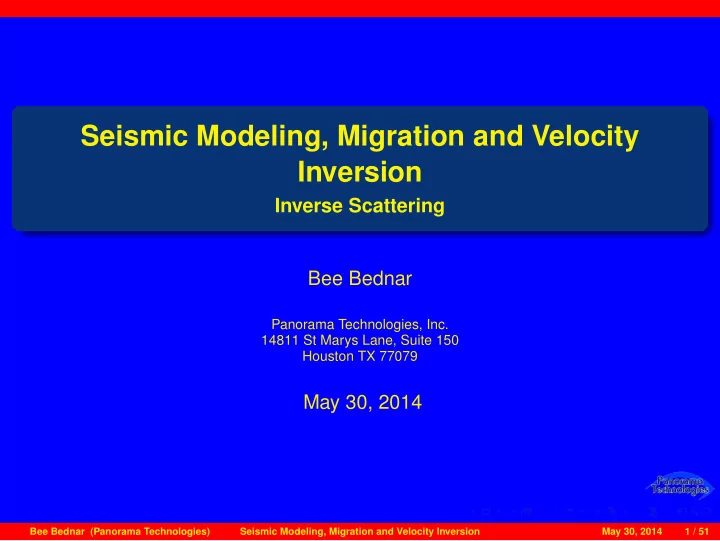
Seismic Modeling, Migration and Velocity Inversion Inverse Scattering Bee Bednar Panorama Technologies, Inc. 14811 St Marys Lane, Suite 150 Houston TX 77079 May 30, 2014 Bee Bednar (Panorama Technologies) Seismic Modeling, Migration and Velocity Inversion May 30, 2014 1 / 51

Outline Fundamental Principles 1 Green’s Functions, Operators, Data and Sources 2 Functions Operators Data and Sources Full Waveform Inversion 3 Operator Form Inverse Scattering 4 The Lippmann-Schwinger Equation The Forward Scattering Series The Inverse Series Convergence Multiple Elimination Internal Multiple Elimination The Final Step Final Comments 5 Bee Bednar (Panorama Technologies) Seismic Modeling, Migration and Velocity Inversion May 30, 2014 2 / 51

Fundamental Principles Outline Fundamental Principles 1 Green’s Functions, Operators, Data and Sources 2 Functions Operators Data and Sources Full Waveform Inversion 3 Operator Form Inverse Scattering 4 The Lippmann-Schwinger Equation The Forward Scattering Series The Inverse Series Convergence Multiple Elimination Internal Multiple Elimination The Final Step Final Comments 5 Bee Bednar (Panorama Technologies) Seismic Modeling, Migration and Velocity Inversion May 30, 2014 3 / 51

Fundamental Principles Fundamental Inversion Principle The fundamental principle underlying the inversion of seismic data is the determination of an Earth model that is fully consistent with measured data. That is, given data U measured over some part of the Earth’s surface, inversion seeks that Earth model whose synthetic seismic response matches the measured data as accurately as possible. Bee Bednar (Panorama Technologies) Seismic Modeling, Migration and Velocity Inversion May 30, 2014 4 / 51

Fundamental Principles Full Waveform Inversion Full waveform inversion is a Newton-Raphson style minimization method. (see e.g. Lailly (1983), Tarantola (1984), Crase (1990), Mora (1987,1999), Pratt (1999), and Pratt and Shipp (1999)) A quantitative difference between measured, for which the underlying mathematical model is not known, and synthetic data, for which a model is known, is minimized. If successful this approach provides a model that is completely consistent withe observed or measured data. Bee Bednar (Panorama Technologies) Seismic Modeling, Migration and Velocity Inversion May 30, 2014 5 / 51

Fundamental Principles Inverse Scattering Inversion Inverse scattering is a step-by-step method in which parts of the original measured data are eliminated until the remaining data consist of primary reflections only. The final step seeks to produce an accurate image with zero knowledge of the primary Earth model. Each step involves identifying and summing a sub series of the full inverse scattering series. There are, of course, sub series sums that focus on other useful information, but these are beyond the scope of this presentation. Bee Bednar (Panorama Technologies) Seismic Modeling, Migration and Velocity Inversion May 30, 2014 6 / 51

Fundamental Principles Full waveform Inversion and Inverse Scattering Alternative approaches to seismic data inversion. FWI minimizes an objective function based on the difference between synthetic and real data Some have called this an indirect method Suggests that it is not worth the research effort it currently enjoys. Inverse scattering is a step-by-step approach the removes all multiples before producing an image of the seismic data without knowledge of the velocity Some consider this to direct method As such it is superior to FWI At first glance the two approaches seem to have sufficiently different theoretical foundations to suggest that they have little in common,but as we will see they both work with residual type data. Bee Bednar (Panorama Technologies) Seismic Modeling, Migration and Velocity Inversion May 30, 2014 7 / 51

Green’s Functions, Operators, Data and Sources Outline Fundamental Principles 1 Green’s Functions, Operators, Data and Sources 2 Functions Operators Data and Sources Full Waveform Inversion 3 Operator Form Inverse Scattering 4 The Lippmann-Schwinger Equation The Forward Scattering Series The Inverse Series Convergence Multiple Elimination Internal Multiple Elimination The Final Step Final Comments 5 Bee Bednar (Panorama Technologies) Seismic Modeling, Migration and Velocity Inversion May 30, 2014 8 / 51

Green’s Functions, Operators, Data and Sources Functions Green’s Function The Green’s function for a simple two-way-frequency-domain-scalar wave equation is defined as the solution to � ω 2 � K + 1 ρ ∇ 2 G ( r , r s , ω ) = − δ ( r − r s ) , where δ is the Dirac delta function, r and r s are the field and source location variables, K is bulk modulus, and ρ is density. In mathematical terms, G is the impulse response of the inhomogeneous differential equation. Bee Bednar (Panorama Technologies) Seismic Modeling, Migration and Velocity Inversion May 30, 2014 9 / 51

Green’s Functions, Operators, Data and Sources Operators Green’s Operators The principle of superposition says that convolution U = G ∗ g of a Green’s function with a source g ( r s , ω ) is the solution to the inhomogeneous equation � ω 2 � K + 1 ρ ∇ 2 U = g ( r s , ω ) so we can think of G as an operator from sources to data. Bee Bednar (Panorama Technologies) Seismic Modeling, Migration and Velocity Inversion May 30, 2014 10 / 51

Green’s Functions, Operators, Data and Sources Operators Differential Equations as Operators If we define the differential operator L as � ω 2 K + 1 � ρ ∇ 2 L = then L is an operator from data back to sources and the corresponding Green’s operator is the negative inverse of L . Thus, LG = − I Bee Bednar (Panorama Technologies) Seismic Modeling, Migration and Velocity Inversion May 30, 2014 11 / 51

Green’s Functions, Operators, Data and Sources Data and Sources Operator Relationships In operator terms, U = G ( φ ) for a source φ satisfies L ( U ) = φ. (1) In this case, U when restricted to a recording surface is what we like to call seismic data and normally is the five-dimensional data set we record on or near the surface. Using modern computational resources, U can be synthesize quite efficiently and in this context measured everywhere on and within the model defining L . Bee Bednar (Panorama Technologies) Seismic Modeling, Migration and Velocity Inversion May 30, 2014 12 / 51

Green’s Functions, Operators, Data and Sources Data and Sources Sources as data and data as sources In what follows, we make no mathematical distinction between U or φ . They are simply well behaved continuous possibly vector valued functions on the same domain. They are differential up to the highest order deemed appropriate and are elements of the same function space. However, because G generates data, and L produces sources, it is convenient to think of the first in terms of sources and the second in terms of data. Bee Bednar (Panorama Technologies) Seismic Modeling, Migration and Velocity Inversion May 30, 2014 13 / 51

Full Waveform Inversion Outline Fundamental Principles 1 Green’s Functions, Operators, Data and Sources 2 Functions Operators Data and Sources Full Waveform Inversion 3 Operator Form Inverse Scattering 4 The Lippmann-Schwinger Equation The Forward Scattering Series The Inverse Series Convergence Multiple Elimination Internal Multiple Elimination The Final Step Final Comments 5 Bee Bednar (Panorama Technologies) Seismic Modeling, Migration and Velocity Inversion May 30, 2014 14 / 51

Full Waveform Inversion The Optimization Problem Full waveform inversion (FWI) is formulated as an optimization problem where an objective function of the form J ( U , U 0 ) (2) is minimized. Here U = G ( φ ) represents recorded data for an unknown L and source φ and U 0 = G 0 ( φ ) represents synthetic data for a known Green’s function. The determination of an accurate version of φ is critical for FWI to be successful. Long offsets and low frequencies are also extremely important. Bee Bednar (Panorama Technologies) Seismic Modeling, Migration and Velocity Inversion May 30, 2014 15 / 51

Full Waveform Inversion The Objective Function In the current research literature, (see Symes (2010)) the function J takes many forms. Most frequently J is the L 2 norm (Pratt (1999), Pratt and Shipp (1999)) , but it can also be an L 1 norm, the norm of a phase difference (Bednar et. al. (2007)), a logarithmic difference (Shin et. al. (2007)), an amplitude difference (Pyun et. al. (2007)), the norm of a difference of analytic functions, or the norm of envelope differences. It has been specified in space-time, frequency, and in the Laplace domain (Shin and Cha (2008)). Bee Bednar (Panorama Technologies) Seismic Modeling, Migration and Velocity Inversion May 30, 2014 16 / 51