Seismic Modeling, Migration and Velocity Inversion Full Waveform - PowerPoint PPT Presentation
Seismic Modeling, Migration and Velocity Inversion Full Waveform Inversion Bee Bednar Panorama Technologies, Inc. 14811 St Marys Lane, Suite 150 Houston TX 77079 May 30, 2014 Bee Bednar (Panorama Technologies) Seismic Modeling, Migration
Seismic Modeling, Migration and Velocity Inversion Full Waveform Inversion Bee Bednar Panorama Technologies, Inc. 14811 St Marys Lane, Suite 150 Houston TX 77079 May 30, 2014 Bee Bednar (Panorama Technologies) Seismic Modeling, Migration and Velocity Inversion May 30, 2014 1 / 53
Outline Prestack Inversion 1 Full Waveform Inversion 2 The Basic Idea The Math 3 Marmousi Example 4 Estimating the Initial Model FWI Bee Bednar (Panorama Technologies) Seismic Modeling, Migration and Velocity Inversion May 30, 2014 2 / 53
Prestack Inversion Outline Prestack Inversion 1 Full Waveform Inversion 2 The Basic Idea The Math 3 Marmousi Example 4 Estimating the Initial Model FWI Bee Bednar (Panorama Technologies) Seismic Modeling, Migration and Velocity Inversion May 30, 2014 3 / 53
Prestack Inversion AVA Based ”Inversion” Prestack inversion is sometimes based on minimizing � � 2 � � S data F ( I P , I S , ρ ) = − S ij ( I P , I S , ρ ) + � R ij ( I P , I S , ρ ) � α ij i , j ij � � � � + � ρ low − ˆ ρ low � − ˆ − ˆ � I low I low � + � I low I low + P P S S j subject to I Pmin ≤ I P ≤ I Pmax I Smin ≤ I S ≤ I Smax ρ min ≤ ρ ≤ ρ max (1) Bee Bednar (Panorama Technologies) Seismic Modeling, Migration and Velocity Inversion May 30, 2014 4 / 53
Prestack Inversion AVA Based ”Inversion” Notes: I P , I S , are P and S impedance and ρ is density in time i is the angle-stack index j is the sample index R ij ( I P , I S , ρ ) is the angle-dependent PP reflectivity S data is the measured AVA amplitude ij S ij ( I P , I S , ρ ) is the 1D numerically simulated synthetic seismic data Variables with low superscripts designate low-frequency components of P-impedance, S-impedance, and density respectively. Bee Bednar (Panorama Technologies) Seismic Modeling, Migration and Velocity Inversion May 30, 2014 5 / 53
Prestack Inversion AVA Based ”Inversion” This is not Full Waveform Inversion Bee Bednar (Panorama Technologies) Seismic Modeling, Migration and Velocity Inversion May 30, 2014 6 / 53
Full Waveform Inversion Outline Prestack Inversion 1 Full Waveform Inversion 2 The Basic Idea The Math 3 Marmousi Example 4 Estimating the Initial Model FWI Bee Bednar (Panorama Technologies) Seismic Modeling, Migration and Velocity Inversion May 30, 2014 7 / 53
Full Waveform Inversion The Basic Idea Full Waveform Inversion For a given model For each observed shot, synthesize data to match the real acquisition Use a full two-way modeling algorithm Save a trace at each model node Compute the difference between the shot and the real data These data are called the residuals Back propagated the residuals into the model Use a full two-way modeling algorithm Save a trace at each model node Preform a shot-profile migration of the residuals The shot is the forward-propagated synthetic The receiver traces are the back-propagated residuals Divide the back by the forward propagated traces Normalize the image above by the velocity squared Add the normalized image to the current model Repeat the previous steps until the norm of the model difference is small FWI is really a iterative migration scheme Bee Bednar (Panorama Technologies) Seismic Modeling, Migration and Velocity Inversion May 30, 2014 8 / 53
The Math Outline Prestack Inversion 1 Full Waveform Inversion 2 The Basic Idea The Math 3 Marmousi Example 4 Estimating the Initial Model FWI Bee Bednar (Panorama Technologies) Seismic Modeling, Migration and Velocity Inversion May 30, 2014 9 / 53
The Math Variational Formulation of the Wave Equation The two-way-frequency-domain-scalar wave equation − ω 2 c 2 − ∇ 2 U = f ( � x s , ω ) , (2) where f ( � x s , ω ) is a compressional source located at � x s , and c ( � x ) is velocity, has the variational form � � ω φ ( U , V ) = − c 2 Vd Ω + ∇ U ∇ Vd Ω = f ( � x s , t ) (3) Ω Ω where V are functions used to approximate U ( x , y , z ) . Bee Bednar (Panorama Technologies) Seismic Modeling, Migration and Velocity Inversion May 30, 2014 10 / 53
The Math The Matrix Form Given a family, V k , of approximating functions s we can approximate U, and f � n � n by u ( � U k V k ( � x ) and f ( � f k V k ( � x ) = x s , ω ) = x ) so that the variational form k = 1 k = 1 in equation (3) � n n � � U k φ ( V k , V j ) = f k V k V j d Ω (4) k = 1 k = 1 Ω can be expressed in matrix form as S � U = M � f (5) Here S is called the complex impedance matrix and M the stiffness matrix. Bee Bednar (Panorama Technologies) Seismic Modeling, Migration and Velocity Inversion May 30, 2014 11 / 53
The Math Notes S � U = M � f is a single frequency equation. The matrix M does not depend on U k . Its more like a new source term. With proper choice of { V k } we can arrange for M = I . For our purposes here and to simplify notation, S � U = � f (6) We assume that S is square, symmetric, and invertible. The inverse, S − 1 , of S is a modeling ”operator” Thus � U = S − 1 � f (7) Bee Bednar (Panorama Technologies) Seismic Modeling, Migration and Velocity Inversion May 30, 2014 12 / 53
The Math Full Waveform Inversion Full waveform inversion begins with a suitably chosen objective function which for the classical case is E = � J ( � D , � U ) � = � � D − � U � . (8) where � · � is the usual least squares norm, � D is the observed seismic data and � U = S − 1 � f is synthetic data corresponding to the current velocity model estimate. Bee Bednar (Panorama Technologies) Seismic Modeling, Migration and Velocity Inversion May 30, 2014 13 / 53
The Math The Inversion Scheme Given an initial velocity model, we can consider two update schemes: Move in the negative direction of the gradient of E . Use the full Newton method (Lines and Treitel 1984) to update the current model. Choosing the second means that our updating scheme immediately takes the form c n = � c n − 1 − H − 1 ∇ � � n − 1 E (9) c Thus, we must calculated the gradient of E and also invert the Hessian matrix H . Bee Bednar (Panorama Technologies) Seismic Modeling, Migration and Velocity Inversion May 30, 2014 14 / 53
The Math The Inversion Scheme cont’d Finding the gradient of the objective function E requires that we find the gradient of � U = S − 1 � f with respect to the sampled velocity model { c k } Thus, U + S ∂� ∂ S U � = 0 (10) ∂ c k ∂ c k ∂� U = S − 1 � P k (11) ∂ c k and P k = − ∂ S � � U (12) ∂ c k where the middle equation defines what is normally called the partial derivative wave field, and the bottom equation defines the so called virtual source vector required to perturb k -th velocity element. Bee Bednar (Panorama Technologies) Seismic Modeling, Migration and Velocity Inversion May 30, 2014 15 / 53
The Math The Inversion Scheme cont’d From the objective function 8 2 � 3 9 ( U 1 − D 1 ) > > > > > � > > 6 ( U 2 − D 2 ) 7 > > > > 6 7 > > > > 6 . 7 > > > . > » ∂ U 1 6 7 > > . > > – 6 7 > ∂ E ∂ U 2 ∂ U nr ∂ U nn < = 6 7 = Re � (13) ( U nr − D nr ) · · · · · · 6 7 ∂ c k ∂ c k ∂ c k ∂ c k ∂ c k 6 7 > > > 6 0 7 > > > > 6 7 > > > . > 6 7 > > . > > 6 7 > . > > > 4 5 > > > > > 0 : ; and from the partial derivative wave field ∂ E n o ( � P k ) T S − 1 � = Re r (14) ∂ c k where i T h � � � � r = ( U 1 − D 1 ) , ( U 2 − D 2 ) , · · · ( U nr − D nr ) , 0 , · · · , 0 (15) Bee Bednar (Panorama Technologies) Seismic Modeling, Migration and Velocity Inversion May 30, 2014 16 / 53
The Math The Inversion Scheme cont’d Finally, we approximate the Hessian via � P k so that for each k, the updating scheme is � � ( � P k ) T S − 1 � Re r � c l + 1 = c l k + α � � (16) k P k ) T � ( � � ω Re P k + λ Bee Bednar (Panorama Technologies) Seismic Modeling, Migration and Velocity Inversion May 30, 2014 17 / 53
Marmousi Example Outline Prestack Inversion 1 Full Waveform Inversion 2 The Basic Idea The Math 3 Marmousi Example 4 Estimating the Initial Model FWI Bee Bednar (Panorama Technologies) Seismic Modeling, Migration and Velocity Inversion May 30, 2014 18 / 53
Marmousi Example Estimating the Initial Model Marmousi MVA (a) Gather Picks (b) Semblance Picks (c) NMO’d Gather Typical Marmousi gather with picks, a semblance panel with picks, and the NMO corrected gather. Bee Bednar (Panorama Technologies) Seismic Modeling, Migration and Velocity Inversion May 30, 2014 19 / 53
Marmousi Example Estimating the Initial Model Marmousi MVA (d) Marmousi Time-RMS model (e) Marmousi Depth-Interval model Initial stacking velocity models in time-RMS (left) and interval-depth (right). Bee Bednar (Panorama Technologies) Seismic Modeling, Migration and Velocity Inversion May 30, 2014 20 / 53
Marmousi Example Estimating the Initial Model Marmousi MVA First iteration Marmousi stacking velocity based Kirchhoff migration. Bee Bednar (Panorama Technologies) Seismic Modeling, Migration and Velocity Inversion May 30, 2014 21 / 53
Recommend
More recommend
Explore More Topics
Stay informed with curated content and fresh updates.
