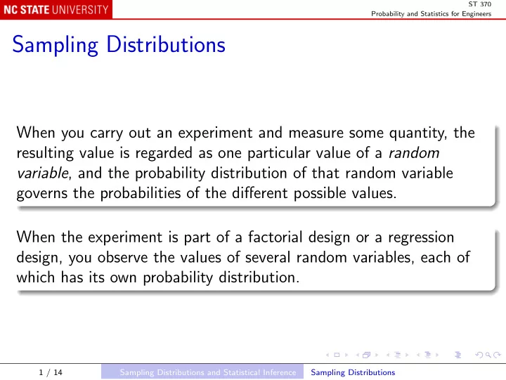
Sampling Distributions When you carry out an experiment and measure - PowerPoint PPT Presentation

ST 370 Probability and Statistics for Engineers Sampling Distributions When you carry out an experiment and measure some quantity, the resulting value is regarded as one particular value of a random variable , and the probability distribution of that random variable governs the probabilities of the different possible values. When the experiment is part of a factorial design or a regression design, you observe the values of several random variables, each of which has its own probability distribution. 1 / 14 Sampling Distributions and Statistical Inference Sampling Distributions

ST 370 Probability and Statistics for Engineers Any quantity calculated from the observed values, such as an estimate of one of the parameters, is called a statistic . Because it is a function of the observed values of random variables, a statistic is also a random variable. As a random variable, a statistic has a probability distribution, called its sampling distribution , and the standard deviation of that distribution is called the standard error of the statistic. The sampling distribution of a parameter estimate is the key to making statistical inferences about the parameter that it estimates. 2 / 14 Sampling Distributions and Statistical Inference Sampling Distributions

ST 370 Probability and Statistics for Engineers Factorial designs Consider for example the replicated two-factor design, for which the statistical model is Y i , j , k = µ + τ i + β j + ( τβ ) i , j + ǫ i , j , k , i = 1 , . . . , a , j = 1 , . . . , b , k = 1 , . . . , n where ǫ i , j , k , i = 1 , . . . , a , j = 1 , . . . , b , k = 1 , . . . , n are independent random variables, each distributed as N (0 , σ 2 ). 3 / 14 Sampling Distributions and Statistical Inference Sampling Distributions

ST 370 Probability and Statistics for Engineers An equivalent way to write the model is: Y i , j , k , i = 1 , . . . , a , j = 1 , . . . , b , k = 1 , . . . , n are independent random variables, normally distributed with common variance σ 2 and expected values E ( Y i , j , k ) = µ + τ i + β j + ( τβ ) i , j , i = 1 , . . . , a , j = 1 , . . . , b , k = 1 , . . . , n 4 / 14 Sampling Distributions and Statistical Inference Sampling Distributions

ST 370 Probability and Statistics for Engineers With constraints such as τ 1 = β 1 = 0 , ( τβ ) i , 1 = 0 , i = 1 , . . . , a and ( τβ ) 1 , j = 0 , j = 1 , . . . , b the least squares estimates of the parameters can be found. 5 / 14 Sampling Distributions and Statistical Inference Sampling Distributions

ST 370 Probability and Statistics for Engineers Regression designs The statistical model is Y i = β 0 + β 1 x i , 1 + · · · + β k x i , k + ǫ i where ǫ i , i = 1 , . . . , n are independent random variables, each distributed as N (0 , σ 2 ). Again, an equivalent way to write the model is: Y i , i = 1 , n , are independent random variables, normally distributed with common variance σ 2 and expected values E ( Y i ) = β 0 + β 1 x i , 1 + · · · + β k x i , k . 6 / 14 Sampling Distributions and Statistical Inference Sampling Distributions

ST 370 Probability and Statistics for Engineers General linear model Any factorial model may be written as a regression model by using indicator variables, so the regression model is the more general form. The key sampling distribution results for the least squares estimates are: Each parameter estimate ˆ β j has a Gaussian distribution, with expected value equal to β j (they are unbiased ). The standard error of each estimate is of the form a j × σ , where a j is a quantity that can be calculated from the design, and does not depend on the unknown parameters. So ˆ β j − β j ∼ N (0 , 1) . a j σ 7 / 14 Sampling Distributions and Statistical Inference Sampling Distributions

ST 370 Probability and Statistics for Engineers The residual mean square s 2 has the property that ν s 2 σ 2 has the chi-squared distribution with ν degrees of freedom, which is a special case of the Gamma distribution. Here ν is the degrees of freedom for residuals. Also, s 2 is independent of the least squares estimates ˆ β j . So ˆ β j − β j T = ∼ Student’s t with ν degrees of freedom a j s The “standard error” reported by software is the estimated standard error a j s . 8 / 14 Sampling Distributions and Statistical Inference Sampling Distributions

ST 370 Probability and Statistics for Engineers Confidence intervals �� � � ˆ β j − β j � � 1 − α = P ( | T | ≤ t α/ 2 ,ν ) = P � ≤ t α/ 2 ,ν � � a j s � � � � ˆ � β j − β j = P − t α/ 2 ,ν ≤ ≤ t α/ 2 ,ν a j s � � − t α/ 2 ,ν × a j s ≤ ˆ = P β j − β j ≤ t α/ 2 ,ν × a j s � � − ˆ β j − t α/ 2 ,ν × a j s ≤ − β j ≤ − ˆ = P β j + t α/ 2 ,ν × a j s � � β j + t α/ 2 ,ν × a j s ≥ β j ≥ ˆ ˆ = P β j − t α/ 2 ,ν × a j s 9 / 14 Sampling Distributions and Statistical Inference Sampling Distributions

ST 370 Probability and Statistics for Engineers That is, the probability that β j lies between the random limits ˆ β j ± t α/ 2 ,ν × a j s is 1 − α , and � � β j − t α/ 2 ,ν × a j s , ˆ ˆ β j + t α/ 2 ,ν × a j s is a 100(1 − α )% confidence interval for β j . 10 / 14 Sampling Distributions and Statistical Inference Sampling Distributions

ST 370 Probability and Statistics for Engineers Hypothesis tests Similarly, under H 0 : β j = β 0 j , the probability of finding as large a value as ˆ β j − β 0 j t obs = a j s is P ( | T | ≥ | t obs | ) where T ∼ Student’s t with ν degrees of freedom. This is the P -value reported by software. 11 / 14 Sampling Distributions and Statistical Inference Sampling Distributions

ST 370 Probability and Statistics for Engineers Nested models Write SS E , reduced and SS E , full for the residual sums of squares of the two models, where the “reduced” model is nested within the “full” model. The extra sum of squares is SS R , extra = SS E , reduced − SS E , full and if this is large, the r additional predictors have explained a substantial additional amount of variability. 12 / 14 Sampling Distributions and Statistical Inference Sampling Distributions

ST 370 Probability and Statistics for Engineers The key properties of these sums of squares are: SS R , extra and SS E , full are independent; SS E , full /σ 2 follows the chi-squared distribution with ν degrees of freedom, where ν is the residual degrees of freedom for the full model. Under the null hypothesis that the added predictors all have zero coefficients, SS R , extra /σ 2 follows the chi-squared distribution, with r degrees of freedom. Consequently, under that null hypothesis, the F -statistic F = SS R , extra / r MS E , full follows Fisher’s F -distribution with r and ν degrees of freedom. 13 / 14 Sampling Distributions and Statistical Inference Sampling Distributions

ST 370 Probability and Statistics for Engineers The “test for significance of regression” is a special case, where the reduced model has no predictors, only an intercept. In this case, and in the general nested model comparison, the P -value reported by software is P ( F ≥ F obs ) where F ∼ Fisher’s F with r and ν degrees of freedom. 14 / 14 Sampling Distributions and Statistical Inference Sampling Distributions