Goodness-of-Fit Tests [Identifying the distribution] Conduct - PowerPoint PPT Presentation
Chapter 9 Input Modeling (3) Banks, Carson, Nelson & Nicol Discrete-Event System Simulation Goodness-of-Fit Tests [Identifying the distribution] Conduct hypothesis testing on input data distribution using: Kolmogorov-Smirnov test
Chapter 9 Input Modeling (3) Banks, Carson, Nelson & Nicol Discrete-Event System Simulation
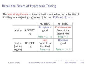
Goodness-of-Fit Tests [Identifying the distribution] Conduct hypothesis testing on input data distribution using: Kolmogorov-Smirnov test Chi-square test No single correct distribution in a real application exists. If very little data are available, it is unlikely to reject any candidate distributions If a lot of data are available, it is likely to reject all candidate distributions 2
Chi-Square test [Goodness-of-Fit Tests] Intuition: comparing the histogram of the data to the shape of the candidate density or mass function Valid for large sample sizes when parameters are estimated by maximum likelihood By arranging the n observations into a set of k class intervals or cells, the test statistics is: k 2 ( O E ) Expected Frequency 2 i i 0 E i = n*p i E i i 1 where p i is the theoretical Observed prob. of the i th interval. Frequency Suggested Minimum = 5 which approximately follows the chi-square distribution with k-s-1 degrees of freedom, where s = # of parameters of the hypothesized distribution estimated by the sample statistics. 3
Chi-Square test [Goodness-of-Fit Tests] The hypothesis of a chi-square test is: H 0 : The random variable, X , conforms to the distributional assumption with the parameter(s) given by the estimate(s). H 1 : The random variable X does not conform. If the distribution tested is discrete and combining adjacent cell is not required (so that E i > minimum requirement): Each value of the random variable should be a class interval, unless combining is necessary, and p p(x ) P(X x ) i i i 4
Chi-Square test [Goodness-of-Fit Tests] If the distribution tested is continuous: a i p f ( x ) dx F ( a ) F ( a ) i i i 1 a i 1 where a i-1 and a i are the endpoints of the i th class interval and f(x) is the assumed pdf, F(x) is the assumed cdf. Recommended number of class intervals ( k ): Sample Size, n Number of Class Intervals, k 20 Do not use the chi-square test 50 5 to 10 100 10 to 20 n 1/2 to n/5 > 100 Caution: Different grouping of data (i.e., k ) can affect the hypothesis testing result. 5
Chi-Square test [Goodness-of-Fit Tests] Vehicle Arrival Example (continued): H 0 : the random variable is Poisson distributed. H 1 : the random variable is not Poisson distributed. (O i - E i ) 2 /E i E np ( x ) x i Observed Frequency, O i Expected Frequency, E i i 0 12 2.6 x 7.87 e 1 10 9.6 n 2 19 17.4 0.15 x ! 3 17 21.1 0.8 4 19 19.2 4.41 5 6 14.0 2.57 6 7 8.5 0.26 7 5 4.4 8 5 2.0 11.62 9 3 0.8 Combined because 10 3 0.3 of min E i > 11 1 0.1 27.68 100 100.0 Degree of freedom is k-s-1 = 7-1-1 = 5 , hence, the hypothesis is rejected at the 0.05 level of significance. 2 2 27 . 68 11 . 1 0 0 . 05 , 5 6
Kolmogorov-Smirnov Test [Goodness-of-Fit Tests] Intuition: formalize the idea behind examining a q-q plot Recall from Chapter 7.4.1: The test compares the continuous cdf, F(x) , of the hypothesized distribution with the empirical cdf, S N (x), of the N sample observations. Based on the maximum difference statistics (Tabulated in A.8): D = max| F(x) - S N (x)| A more powerful test, particularly useful when: Sample sizes are small, No parameters have been estimated from the data. 7
Kolmogorov-Smirnov Test Compares the continuous cdf, F(x) , of the uniform distribution with the empirical cdf, S N (x), of the N sample observations. We know: F ( x ) x , 0 x 1 If the sample from the RN generator is R 1 , R 2 , …, R N , then the empirical cdf, S N (x) is: number of R , R ,..., R which are x 1 2 n S ( x ) N N Based on the statistic: D = max| F(x) - S N (x)| Sampling distribution of D is known (a function of N , tabulated in Table A.8.) A more powerful test, recommended. 8
Kolmogorov-Smirnov Test Example: Suppose 5 generated numbers are 0.44, 0.81, 0.14, 0.05, 0.93 . Arrange R (i) from R (i) 0.05 0.14 0.44 0.81 0.93 smallest to largest Step 1: i/N 0.20 0.40 0.60 0.80 1.00 D + = max {i/N – R (i) } i/N – R (i) 0.15 0.26 0.16 0.01 0.07 Step 2: R (i) – (i-1)/N 0.05 0.06 0.04 0.21 0.13 D - = max {R (i) - (i-1)/N} Step 3: D = max(D + , D - ) = 0.26 Step 4: For = 0.05 , D = 0.565 > D Hence, H 0 is not rejected. 9
p- Values and “Best Fits” [Goodness-of-Fit Tests] p-value for the test statistics The significance level at which one would just reject H 0 for the given test statistic value. A measure of fit, the larger the better Large p-value : good fit Small p-value : poor fit Vehicle Arrival Example (cont.): H 0 : data is Possion 0 2 Test statistics: , with 5 degrees of freedom 27 . 68 p-value = 0.00004 , meaning we would reject H 0 with 0.00004 significance level, hence Poisson is a poor fit. 10
p- Values and “Best Fits” [Goodness-of-Fit Tests] Many software use p-value as the ranking measure to automatically determine the “best fit”. Things to be cautious about: Software may not know about the physical basis of the data, distribution families it suggests may be inappropriate. Close conformance to the data does not always lead to the most appropriate input model. p-value does not say much about where the lack of fit occurs Recommended: always inspect the automatic selection using graphical methods. 11
Fitting a Non-stationary Poisson Process Fitting a NSPP to arrival data is difficult, possible approaches: Fit a very flexible model with lots of parameters or Approximate constant arrival rate over some basic interval of time, but vary it from time interval to time interval. Our focus Suppose we need to model arrivals over time [0,T], our approach is the most appropriate when we can: Observe the time period repeatedly and Count arrivals / record arrival times. 12
Fitting a Non-stationary Poisson Process The estimated arrival rate during the i th time period is: n 1 ˆ ( t ) C D ij n t j 1 where n = # of observation periods, D t = time interval length C ij = # of arrivals during the i th time interval on the j th observation period Example: Divide a 10 -hour business day [ 8am,6pm ] into equal intervals k = 20 whose length D t = ½ , and observe over n =3 days Number of Arrivals Estimated Arrival Day 1 Day 2 Day 3 Time Period Rate (arrivals/hr) For instance, 8:00 - 8:00 12 14 10 24 1/3(0.5)*(23+26+32) 8:30 - 9:00 23 26 32 54 = 54 arrivals/hour 9:00 - 9:30 27 18 32 52 9:30 - 10:00 20 13 12 30 13
Selecting Model without Data If data is not available, some possible sources to obtain information about the process are: Engineering data: often product or process has performance ratings provided by the manufacturer or company rules specify time or production standards. Expert option: people who are experienced with the process or similar processes, often, they can provide optimistic, pessimistic and most-likely times, and they may know the variability as well. Physical or conventional limitations: physical limits on performance, limits or bounds that narrow the range of the input process. The nature of the process. The uniform, triangular, and beta distributions are often used as input models. 14
Covariance and Correlation [Multivariate/Time Series] Consider the model that describes relationship between X 1 and X 2 : b ( X ) ( X ) is a random variable 1 1 2 2 with mean 0 and is b = 0, X 1 and X 2 are statistically independent independent of X 2 b > 0, X 1 and X 2 tend to be above or below their means together b < 0, X 1 and X 2 tend to be on opposite sides of their means Covariance between X 1 and X 2 : cov( X , X ) E [( X )( X )] E ( X X ) 1 2 1 1 2 2 1 2 1 2 = 0 , = 0 then b where c ov ( X 1 , X 2 ) < 0 , < 0 > 0 , > 0 15
Covariance and Correlation [Multivariate/Time Series] Correlation between X 1 and X 2 (values between -1 and 1 ) : cov( , ) X X r 1 2 corr ( X , X ) 1 2 1 2 = 0 , = 0 then b where c orr ( X 1 , X 2 ) < 0 , < 0 > 0 , > 0 The closer r is to -1 or 1 , the stronger the linear relationship is between X 1 and X 2 . 16
Summary In this chapter, we described the 4 steps in developing input data models: Collecting the raw data Identifying the underlying statistical distribution Estimating the parameters Testing for goodness of fit 17
Recommend
More recommend
Explore More Topics
Stay informed with curated content and fresh updates.
