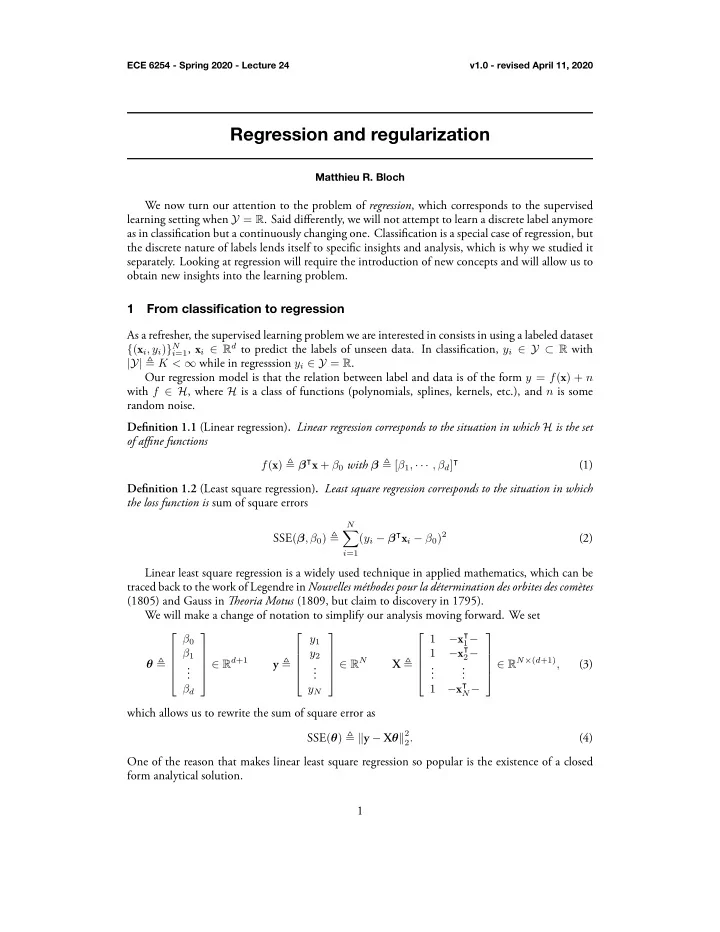
Regression and regularization Matthieu R. Bloch learning setting - PDF document

1 random noise. traced back to the work of Legendre in Nouvelles méthodes pour la détermination des orbites des comètes Linear least square regression is a widely used technique in applied mathematics, which can be (2) . . . . . the loss function is sum of square errors Definition 1.2 (Least square regression) . Least square regression corresponds to the situation in which (1) . of affine functions . . We will make a change of notation to simplify our analysis moving forward. We set separately. Looking at regression will require the introduction of new concepts and will allow us to form analytical solution. One of the reason that makes linear least square regression so popular is the existence of a closed We now turn our attention to the problem of regression , which corresponds to the supervised (4) as in classification but a continuously changing one. Classification is a special case of regression, but the discrete nature of labels lends itself to specific insights and analysis, which is why we studied it obtain new insights into the learning problem. . which allows us to rewrite the sum of square error as (3) As a refresher, the supervised learning problem we are interested in consists in using a labeled dataset . . . (1805) and Gauss in Tieoria Motus (1809, but claim to discovery in 1795). ECE 6254 - Spring 2020 - Lecture 24 v1.0 - revised April 11, 2020 Regression and regularization Matthieu R. Bloch learning setting when Y = R . Said differently, we will not attempt to learn a discrete label anymore 1 From classification to regression { ( x i , y i ) } N i =1 , x i ∈ R d to predict the labels of unseen data. In classification, y i ∈ Y ⊂ R with |Y| ≜ K < ∞ while in regresssion y i ∈ Y = R . Our regression model is that the relation between label and data is of the form y = f ( x ) + n with f ∈ H , where H is a class of functions (polynomials, splines, kernels, etc.), and n is some Definition 1.1 (Linear regression) . Linear regression corresponds to the situation in which H is the set f ( x ) ≜ β ⊺ x + β 0 with β ≜ [ β 1 , · · · , β d ] ⊺ N � ( y i − β ⊺ x i − β 0 ) 2 SSE ( β , β 0 ) ≜ i =1 − x ⊺       1 1 − β 0 y 1 − x ⊺ 1 2 − β 1 y 2       θ ≜   ∈ R d +1  y ≜    ∈ R N X ≜    ∈ R N × ( d +1) ,          − x ⊺ N − β d y N 1 SSE ( θ ) ≜ � y − X θ � 2 2 .

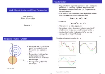
2 (6) random. Fig. 1 shows the resulting predictor obtained by fitting the data to a polynomial of degree Figure 1: Illustration of overfitting (a) True model and sample points. (5) Proof. See annotated slides. when there are too many degrees of freedom in model so that one “learns the noise ” but also when sample error is small, i.e., the underlying model learned generalized poorly. Tiis happens no only Overfitting is the problem that happens when fitting the data well no longer ensures that the out-of- (7) As for classification, linear methods have their limit, and one can create a non-linear estimator linear map ECE 6254 - Spring 2020 - Lecture 24 v1.0 - revised April 11, 2020 Lemma 1.3 (Linear least square solution) . If X ⊺ X is non singular the minimizer of the SSE is θ = ( X ⊺ X ) − 1 X ⊺ y ˆ ■ Tie existence of this solution is a bit misleading because computing ˆ θ can be extremely numer- ically unstable. Tie matrix ( X ⊺ X ) − 1 could be ill-conditioned. using a non-linear feature map Φ : R d → R ℓ : x �→ Φ( x ) . Tie regression model becomes y = β ⊺ Φ( x ) + β 0 with β ∈ R ℓ . Example 1.4. To obtain a least square estimate of cubic polynomial f with d = 1 , one can use the non   1 x   Φ : R → R 4 : x �→  .   x 2  x 3 2 Overfitting and regularization the hypothesis set contains simpler functions than the target function f but the number of sample points N is too small. In general, overfitting occurs as the number of features d begins to approach the number of observations N . To illustrate this, consider the following example in data is generated as y = x 2 + n with x ∈ [ − 1; 1] , where n ∼ N (0 , σ = 0 . 1) . We perform regression with polynomial of degree d . Fig. 1a shows the true underlying model and five samples obtained independently and uniformly at True model and data 1.0 1.0 True model degree 4 noisy data 0.8 0.8 0.6 0.6 y y 0.4 0.4 0.2 0.2 True model noisy data 0.0 0.0 1.00 0.75 0.50 0.25 0.00 0.25 0.50 0.75 1.00 1.00 0.75 0.50 0.25 0.00 0.25 0.50 0.75 1.00 x x (b) Regression fit with d = 4 . d = 4 . Since we only have five points, there exists a degree four polynomial that predicts exactly the

3 sampled points. value of all five training point. Tiis is an example where our regression is effectively learning the points is small. Tie key solution is a technique called regularization . results for twenty randomly sampled sets of five points. In practice though, we are often interested in limiting overfitting even when the number of data Figure 3: Regression with enough data points domly sampled points. domly sampled points. overfitting disappears once we have enough data points. of the polynomial is one less than the true model so that the model cannot fit the noise; however, unstable prediction that does not generalize well. Perhaps surprisingly, one observes a similar vari- As you can see, there is a huge variance in the resulting predictor, suggesting that we have an Figure 2: Regression with too few datapoints sampled points. ECE 6254 - Spring 2020 - Lecture 24 v1.0 - revised April 11, 2020 noise in the model. To fully appreciate the consequence of overfitting, Fig. 2a shows the regression True model and prediction True model and prediction 1.0 1.0 True model 0.8 0.8 0.6 0.6 0.4 0.4 y y 0.2 0.2 0.0 0.0 True model 0.2 0.2 1.00 0.75 0.50 0.25 0.00 0.25 0.50 0.75 1.00 1.00 0.75 0.50 0.25 0.00 0.25 0.50 0.75 1.00 x x (a) Many regressions with d = 4 on five randomly (b) Many regressions with d = 1 on five randomly ance when trying to fig the data to a polynomial of degree d = 1 . In the latter situation, the degree the variance stems from the fact that there are few sample points. As shown in Fig. 3a and Fig. 3b, True model and prediction True model and prediction 1.0 1.0 0.8 0.8 0.6 0.6 0.4 0.4 y y 0.2 0.2 0.0 0.0 True model True model 0.2 0.2 1.00 0.75 0.50 0.25 0.00 0.25 0.50 0.75 1.00 1.00 0.75 0.50 0.25 0.00 0.25 0.50 0.75 1.00 x x (a) Many regressions with d = 4 on fifty ran- (b) Many regressions with d = 1 on fifty ran-

4 . . . Proof. See annotated slides. (9) ... ... Tikhonov regularization is Lemma 3.1 (Tikhonov regularization solution) . Tie minimizer of the least-square problem with (8) (10) . . (11) same situation as earlier. Notice how the variance of the regression is substantially reduced. randomly sampled points. randomly sampled points. Figure 4: Ridge regression It is also useful to understand Tikhonov regularization as a constrained optimization problem. . ECE 6254 - Spring 2020 - Lecture 24 v1.0 - revised April 11, 2020 3 Tikhonov regularization Tie key idea behind regularization is to introduce a penalty term to “regularize” the vector θ : � y − X θ � 2 2 + � Γ θ � 2 θ = argmin 2 θ where Γ ∈ R ( d +1) × ( d +1) θ = ( X ⊺ X + Γ ⊺ Γ ) − 1 X ⊺ y ˆ ■ √ For the special case Γ = λ I for some λ > 0 , we obtain θ = ( X ⊺ X + λ I ) − 1 X ⊺ y ˆ Tiis simple change has many benefits, including improving numerical stability when computing ˆ θ since X ⊺ X + λ I is better conditioned than X ⊺ X . Ridge regression is a slight variant of the above that does not penalize β 0 and corresponds to   0 0 · · · 0 √ 0 λ · · · 0     Γ =     √ 0 · · · · · · λ To appreciate the effect of regularization. Fig. 4 shows the resulting regressions with λ = 1 in the True model and prediction True model and prediction 1.0 1.0 0.8 0.8 0.6 0.6 0.4 0.4 y y 0.2 0.2 0.0 0.0 True model True model 0.2 0.2 1.00 0.75 0.50 0.25 0.00 0.25 0.50 0.75 1.00 1.00 0.75 0.50 0.25 0.00 0.25 0.50 0.75 1.00 x x (a) Many ridge regressions with d = 4 on five (b) Many ridge regressions with d = 1 on five