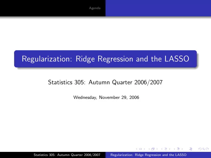
Regularization: Ridge Regression and the LASSO Statistics 305: - - PowerPoint PPT Presentation

Agenda

Regularization: Ridge Regression and the LASSO

Statistics 305: Autumn Quarter 2006/2007

Wednesday, November 29, 2006

Statistics 305: Autumn Quarter 2006/2007 Regularization: Ridge Regression and the LASSO

Agenda

Agenda

1 The Bias-Variance Tradeoff 2 Ridge Regression

Solution to the ℓ2 problem Data Augmentation Approach Bayesian Interpretation The SVD and Ridge Regression

3 Cross Validation

K-Fold Cross Validation Generalized CV

4 The LASSO 5 Model Selection, Oracles, and the Dantzig Selector 6 References Statistics 305: Autumn Quarter 2006/2007 Regularization: Ridge Regression and the LASSO

Part I: The Bias-Variance Tradeoff

Part I The Bias-Variance Tradeoff

Statistics 305: Autumn Quarter 2006/2007 Regularization: Ridge Regression and the LASSO

Part I: The Bias-Variance Tradeoff

Estimating β

As usual, we assume the model: y = f (z) + ε, ε ∼ (0, σ2) In regression analysis, our major goal is to come up with some good regression function ˆ f (z) = z⊤ ˆ β So far, we’ve been dealing with ˆ β

ls, or the least squares

solution:

ˆ β

ls has well known properties (e.g., Gauss-Markov, ML)

But can we do better?

Statistics 305: Autumn Quarter 2006/2007 Regularization: Ridge Regression and the LASSO

Part I: The Bias-Variance Tradeoff

Choosing a good regression function

Suppose we have an estimator ˆ f (z) = z⊤ˆ β To see if ˆ f (z) = z⊤ˆ β is a good candidate, we can ask

• urselves two questions:

1.) Is ˆ β close to the true β? 2.) Will ˆ f (z) fit future observations well?

Statistics 305: Autumn Quarter 2006/2007 Regularization: Ridge Regression and the LASSO

Part I: The Bias-Variance Tradeoff

1.) Is ˆ β close to the true β?

To answer this question, we might consider the mean squared error of our estimate ˆ β:

i.e., consider squared distance of ˆ β to the true β: MSE(ˆ β) = E[||ˆ β − β||2] = E[(ˆ β − β)⊤(ˆ β − β)]

Example: In least squares (LS), we now that: E[(ˆ β

ls − β)⊤(ˆ

β

ls − β)] = σ2tr[(Z⊤Z)−1]

Statistics 305: Autumn Quarter 2006/2007 Regularization: Ridge Regression and the LASSO

Part I: The Bias-Variance Tradeoff

2.) Will ˆ f (z) fit future observations well?

Just because ˆ f (z) fits our data well, this doesn’t mean that it will be a good fit to new data In fact, suppose that we take new measurements y ′

i at the

same zi’s: (z1, y ′

1), (z2, y ′ 2), . . . , (zn, y ′ n)

So if ˆ f (·) is a good model, then ˆ f (zi) should also be close to the new target y ′

i

This is the notion of prediction error (PE)

Statistics 305: Autumn Quarter 2006/2007 Regularization: Ridge Regression and the LASSO

Part I: The Bias-Variance Tradeoff

Prediction error and the bias-variance tradeoff

So good estimators should, on average have, small prediction errors Let’s consider the PE at a particular target point z0 (see the board for a derivation): PE(z0) = EY |Z=z0{(Y − ˆ f (Z))2|Z = z0} = σ2

ε + Bias2(ˆ

f (z0)) + Var(ˆ f (z0)) Such a decomposition is known as the bias-variance tradeoff

As model becomes more complex (more terms included), local structure/curvature can be picked up But coefficient estimates suffer from high variance as more terms are included in the model

So introducing a little bias in our estimate for β might lead to a substantial decrease in variance, and hence to a substantial decrease in PE

Statistics 305: Autumn Quarter 2006/2007 Regularization: Ridge Regression and the LASSO

Part I: The Bias-Variance Tradeoff

Depicting the bias-variance tradeoff

Model Complexity Squared Error

Bias−Variance Tradeoff

Prediction Error Bias^2 Variance

Figure: A graph depicting the bias-variance tradeoff.

Statistics 305: Autumn Quarter 2006/2007 Regularization: Ridge Regression and the LASSO

Part II: Ridge Regression

Part II Ridge Regression

Statistics 305: Autumn Quarter 2006/2007 Regularization: Ridge Regression and the LASSO

Part II: Ridge Regression

• 1. Solution to the ℓ2 Problem and Some Properties
• 2. Data Augmentation Approach
• 3. Bayesian Interpretation
• 4. The SVD and Ridge Regression

Ridge regression as regularization

If the βj’s are unconstrained...

They can explode And hence are susceptible to very high variance

To control variance, we might regularize the coefficients

i.e., Might control how large the coefficients grow

Might impose the ridge constraint: minimize

n

• i=1

(yi − β⊤zi)2 s.t.

p

• j=1

β2

j ≤ t

⇔ minimize (y − Zβ)⊤(y − Zβ) s.t.

p

• j=1

β2

j ≤ t

By convention (very important!):

Z is assumed to be standardized (mean 0, unit variance) y is assumed to be centered

Statistics 305: Autumn Quarter 2006/2007 Regularization: Ridge Regression and the LASSO

Part II: Ridge Regression

• 1. Solution to the ℓ2 Problem and Some Properties
• 2. Data Augmentation Approach
• 3. Bayesian Interpretation
• 4. The SVD and Ridge Regression

Ridge regression: ℓ2-penalty

Can write the ridge constraint as the following penalized residual sum of squares (PRSS): PRSS(β)ℓ2 =

n

• i=1

(yi − z⊤

i β)2 + λ p

• j=1

β2

j

= (y − Zβ)⊤(y − Zβ) + λ||β||2

2

Its solution may have smaller average PE than ˆ β

ls

PRSS(β)ℓ2 is convex, and hence has a unique solution Taking derivatives, we obtain: ∂PRSS(β)ℓ2 ∂β = −2Z⊤(y − Zβ) + 2λβ

Statistics 305: Autumn Quarter 2006/2007 Regularization: Ridge Regression and the LASSO

Part II: Ridge Regression

• 1. Solution to the ℓ2 Problem and Some Properties
• 2. Data Augmentation Approach
• 3. Bayesian Interpretation
• 4. The SVD and Ridge Regression

The ridge solutions

The solution to PRSS(ˆ β)ℓ2 is now seen to be: ˆ βridge

λ

= (Z⊤Z + λIp)−1Z⊤y

Remember that Z is standardized y is centered

Solution is indexed by the tuning parameter λ (more on this later) Inclusion of λ makes problem non-singular even if Z⊤Z is not invertible

This was the original motivation for ridge regression (Hoerl and Kennard, 1970)

Statistics 305: Autumn Quarter 2006/2007 Regularization: Ridge Regression and the LASSO

Part II: Ridge Regression

• 1. Solution to the ℓ2 Problem and Some Properties
• 2. Data Augmentation Approach
• 3. Bayesian Interpretation
• 4. The SVD and Ridge Regression

Tuning parameter λ

Notice that the solution is indexed by the parameter λ

So for each λ, we have a solution Hence, the λ’s trace out a path of solutions (see next page)

λ is the shrinkage parameter

λ controls the size of the coefficients λ controls amount of regularization As λ ↓ 0, we obtain the least squares solutions As λ ↑ ∞, we have ˆ β

ridge λ=∞ = 0 (intercept-only model)

Statistics 305: Autumn Quarter 2006/2007 Regularization: Ridge Regression and the LASSO

Part II: Ridge Regression

• 1. Solution to the ℓ2 Problem and Some Properties
• 2. Data Augmentation Approach
• 3. Bayesian Interpretation
• 4. The SVD and Ridge Regression

Ridge coefficient paths

The λ’s trace out a set of ridge solutions, as illustrated below

DF Coefficient 2 4 6 8 10 age sex bmi map tc ldl hdl tch ltg glu

Ridge Regression Coefficient Paths

Figure: Ridge coefficient path for the diabetes data set found in the lars library in R.

Statistics 305: Autumn Quarter 2006/2007 Regularization: Ridge Regression and the LASSO

Part II: Ridge Regression

• 1. Solution to the ℓ2 Problem and Some Properties
• 2. Data Augmentation Approach
• 3. Bayesian Interpretation
• 4. The SVD and Ridge Regression

Choosing λ

Need disciplined way of selecting λ: That is, we need to “tune” the value of λ In their original paper, Hoerl and Kennard introduced ridge traces:

Plot the components of ˆ β

ridge λ

against λ Choose λ for which the coefficients are not rapidly changing and have “sensible” signs No objective basis; heavily criticized by many

Standard practice now is to use cross-validation (defer discussion until Part 3)

Statistics 305: Autumn Quarter 2006/2007 Regularization: Ridge Regression and the LASSO

Part II: Ridge Regression

• 1. Solution to the ℓ2 Problem and Some Properties
• 2. Data Augmentation Approach
• 3. Bayesian Interpretation
• 4. The SVD and Ridge Regression

Proving that ˆ β

ridge λ

is biased

Let R = Z⊤Z Then: ˆ β

ridge λ

= (Z⊤Z + λIp)−1Z⊤y = (R + λIp)−1R(R−1Z⊤y) = [R(Ip + λR−1)]−1R[(Z⊤Z)−1Z⊤y] = (Ip + λR−1)−1R−1Rˆ β

ls

= (Ip + λR−1)ˆ β

ls

So: E(ˆ β

ridge λ

) = E{(Ip + λR−1)ˆ β

ls}

= (Ip + λR−1)β

(if λ=0)

= β.

Statistics 305: Autumn Quarter 2006/2007 Regularization: Ridge Regression and the LASSO

Part II: Ridge Regression

• 1. Solution to the ℓ2 Problem and Some Properties
• 2. Data Augmentation Approach
• 3. Bayesian Interpretation
• 4. The SVD and Ridge Regression

Data augmentation approach

The ℓ2 PRSS can be written as: PRSS(β)ℓ2 =

n

• i=1

(yi − z⊤

i β)2 + λ p

• j=1

β2

j

=

n

• i=1

(yi − z⊤

i β)2 + p

• j=1

(0 − √ λβj)2 Hence, the ℓ2 criterion can be recast as another least squares problem for another data set

Statistics 305: Autumn Quarter 2006/2007 Regularization: Ridge Regression and the LASSO

Part II: Ridge Regression

• 1. Solution to the ℓ2 Problem and Some Properties
• 2. Data Augmentation Approach
• 3. Bayesian Interpretation
• 4. The SVD and Ridge Regression

Data augmentation approach continued

The ℓ2 criterion is the RSS for the augmented data set: Zλ =                z1,1 z1,2 z1,3 · · · z1,p . . . . . . . . . . . . . . . zn,1 zn,2 zn,3 · · · zn,p √ λ · · · √ λ · · · √ λ ... ... √ λ                ; yλ =               y1 . . . yn . . .               So: Zλ =

• Z

√ λIp

• yλ =

y

• Statistics 305: Autumn Quarter 2006/2007

Regularization: Ridge Regression and the LASSO

Part II: Ridge Regression

• 1. Solution to the ℓ2 Problem and Some Properties
• 2. Data Augmentation Approach
• 3. Bayesian Interpretation
• 4. The SVD and Ridge Regression

Solving the augmented data set

So the “least squares” solution for the augmented data set is: (Z⊤

λ Zλ)−1Z⊤ λ yλ

=

• (Z⊤,

√ λIp)

• Z

√ λIp −1 (Z⊤, √ λIp) y

• =

(Z⊤Z + λIp)−1Z⊤y, which is simply the ridge solution

Statistics 305: Autumn Quarter 2006/2007 Regularization: Ridge Regression and the LASSO

Part II: Ridge Regression

• 1. Solution to the ℓ2 Problem and Some Properties
• 2. Data Augmentation Approach
• 3. Bayesian Interpretation
• 4. The SVD and Ridge Regression

Bayesian framework

Suppose we imposed a multivariate Gaussian prior for β: β ∼ N

• 0, 1

2p Ip

• Then the posterior mean (and also posterior mode) of β is:

βridge

λ

= (Z⊤Z + λIp)−1Z⊤y

Statistics 305: Autumn Quarter 2006/2007 Regularization: Ridge Regression and the LASSO

Part II: Ridge Regression

• 1. Solution to the ℓ2 Problem and Some Properties
• 2. Data Augmentation Approach
• 3. Bayesian Interpretation
• 4. The SVD and Ridge Regression

Computing the ridge solutions via the SVD

Recall ˆ β

ridge λ

= (Z⊤Z + λIp)−1Z⊤y When computing ˆ β

ridge λ

numerically, matrix inversion is avoided:

Inverting Z⊤Z can be computationally expensive: O(p3)

Rather, the singular value decomposition is utilized; that is, Z = UDV⊤, where:

U = (u1, u2, . . . , up) is an n × p orthogonal matrix D = diag(d1, d2, . . . , ≥ dp) is a p × p diagonal matrix consisting of the singular values d1 ≥ d2 ≥ · · · dp ≥ 0 V⊤ = (v⊤

1 , v⊤ 2 , . . . , v⊤ p ) is a p × p matrix orthogonal matrix

Statistics 305: Autumn Quarter 2006/2007 Regularization: Ridge Regression and the LASSO

Part II: Ridge Regression

• 1. Solution to the ℓ2 Problem and Some Properties
• 2. Data Augmentation Approach
• 3. Bayesian Interpretation
• 4. The SVD and Ridge Regression

Numerical computation of ˆ β

ridge λ

Will show on the board that: ˆ β

ridge λ

= (Z⊤Z + λIp)−1Z⊤y = V diag

• dj

d2

j + λ

• U⊤y

Result uses the eigen (or spectral) decomposition of Z⊤Z: Z⊤Z = (UDV⊤)⊤(UDV⊤) = VD⊤U⊤UDV⊤ = VD⊤DV⊤ = VD2V⊤

Statistics 305: Autumn Quarter 2006/2007 Regularization: Ridge Regression and the LASSO

Part II: Ridge Regression

• 1. Solution to the ℓ2 Problem and Some Properties
• 2. Data Augmentation Approach
• 3. Bayesian Interpretation
• 4. The SVD and Ridge Regression

ˆ yridge

λ

and principal components

A consequence is that: ˆ yridge = Zˆ β

ridge λ

=

p

• j=1
• uj

d2

j

d2

j + λu⊤ j

• y

Ridge regression has a relationship with principal components analysis (PCA):

Fact: The derived variable γj = Zvj = ujdj is the jth principal component (PC) of Z Hence, ridge regression projects y onto these components with large dj Ridge regression shrinks the coefficients of low-variance components

Statistics 305: Autumn Quarter 2006/2007 Regularization: Ridge Regression and the LASSO

Part II: Ridge Regression

• 1. Solution to the ℓ2 Problem and Some Properties
• 2. Data Augmentation Approach
• 3. Bayesian Interpretation
• 4. The SVD and Ridge Regression

Orthonormal Z in ridge regression

If Z is orthonormal, then Z⊤Z = Ip, then a couple of closed form properties exist Let ˆ β

ls denote the LS solution for our orthonormal Z; then

ˆ β

ridge λ

= 1 1 + λ ˆ β

ls

The optimal choice of λ minimizing the expected prediction error is: λ∗ = pσ2 p

j=1 β2 j

, where β = (β1, β2, . . . , βp) is the true coefficient vector

Statistics 305: Autumn Quarter 2006/2007 Regularization: Ridge Regression and the LASSO

Part II: Ridge Regression

• 1. Solution to the ℓ2 Problem and Some Properties
• 2. Data Augmentation Approach
• 3. Bayesian Interpretation
• 4. The SVD and Ridge Regression

Smoother matrices and effective degrees of freedom

A smoother matrix S is a linear operator satisfying: ˆ y = Sy

Smoothers put the “hats” on y So the fits are a linear combination of the yi’s, i = 1, . . . , n

Example: In ordinary least squares, recall the hat matrix H = Z(Z⊤Z)−1Z⊤

For rank(Z) = p, we know that tr(H) = p, which is how many degrees of freedom are used in the model

By analogy, define the effective degrees of freedom (or effective number of parameters) for a smoother to be: df(S) = tr(S)

Statistics 305: Autumn Quarter 2006/2007 Regularization: Ridge Regression and the LASSO

Part II: Ridge Regression

• 1. Solution to the ℓ2 Problem and Some Properties
• 2. Data Augmentation Approach
• 3. Bayesian Interpretation
• 4. The SVD and Ridge Regression

Degrees of freedom for ridge regression

In ridge regression, the fits are given by: ˆ y = Z(Z⊤Z + λIp)−1Z⊤y So the smoother or “hat” matrix in ridge takes the form: Sλ = Z(Z⊤Z + λIp)−1Z⊤ So the effective degrees of freedom in ridge regression are given by: df(λ) = tr(Sλ) = tr[Z(Z⊤Z + λIp)−1Z⊤] =

p

• j=1

d2

j

d2

j + λ

Note that df(λ) is monotone decreasing in λ Question: What happens when λ = 0?

Statistics 305: Autumn Quarter 2006/2007 Regularization: Ridge Regression and the LASSO

Part III: Cross Validation

Part III Cross Validation

Statistics 305: Autumn Quarter 2006/2007 Regularization: Ridge Regression and the LASSO

Part III: Cross Validation

• 1. K-Fold Cross Validation
• 2. Generalized CV

How do we choose λ?

We need a disciplined way of choosing λ Obviously want to choose λ that minimizes the mean squared error Issue is part of the bigger problem of model selection

Statistics 305: Autumn Quarter 2006/2007 Regularization: Ridge Regression and the LASSO

Part III: Cross Validation

• 1. K-Fold Cross Validation
• 2. Generalized CV

Training sets versus test sets

If we have a good model, it should predict well when we have new data In machine learning terms, we compute our statistical model ˆ f (·) from the training set A good estimator ˆ f (·) should then perform well on a new, independent set of data We “test” or assess how well ˆ f (·) performs on the new data, which we call the test set

Statistics 305: Autumn Quarter 2006/2007 Regularization: Ridge Regression and the LASSO

Part III: Cross Validation

• 1. K-Fold Cross Validation
• 2. Generalized CV

More on training and testing

Ideally, we would separate our available data into both training and test sets

Of course, this is not always possible, especially if we have a few observations

Hope to come up with the best-trained algorithm that will stand up to the test

Example: The Netflix contest (http://www.netflixprize.com/)

How can we try to find the best-trained algorithm?

Statistics 305: Autumn Quarter 2006/2007 Regularization: Ridge Regression and the LASSO

Part III: Cross Validation

• 1. K-Fold Cross Validation
• 2. Generalized CV

K-fold cross validation

Most common approach is K-fold cross validation:

(i) Partition the training data T into K separate sets of equal size

Suppose T = (T1, T2, . . . , TK) Commonly chosen K’s are K = 5 and K = 10

(ii) For each k = 1, 2, . . ., K, fit the model ˆ f (λ)

−k (z) to the training

set excluding the kth-fold Tk (iii) Compute the fitted values for the observations in Tk, based on the training data that excluded this fold (iv) Compute the cross-validation (CV) error for the k-th fold: (CV Error)(λ)

k

= |Tk|−1

• (z,y)∈Tk

(y − ˆ f (λ)

−k (z))2

Statistics 305: Autumn Quarter 2006/2007 Regularization: Ridge Regression and the LASSO

Part III: Cross Validation

• 1. K-Fold Cross Validation
• 2. Generalized CV

K-fold cross validation (continued)

The model then has overall cross-validation error: (CV Error)(λ) = K −1

K

• k=1

(CV Error)(λ)

k

Select λ∗ as the one with minimum (CV Error)(λ) Compute the chosen model ˆ f (z)(λ∗) on the entire training set T = (T1, T2, . . . , Tk) Apply ˆ f (z)(λ∗) to the test set to assess test error

Statistics 305: Autumn Quarter 2006/2007 Regularization: Ridge Regression and the LASSO

Part III: Cross Validation

• 1. K-Fold Cross Validation
• 2. Generalized CV

Plot of CV errors and standard error bands

30 35 40 45 50 55 0.16 0.18 0.20 0.22 0.24

CV Bands from a Ridge Regression on Spam Data

df Squared Error

Figure: Cross validation errors from a ridge regression example on spam data.

Statistics 305: Autumn Quarter 2006/2007 Regularization: Ridge Regression and the LASSO

Part III: Cross Validation

• 1. K-Fold Cross Validation
• 2. Generalized CV

Cross validation with few observations

Remark: Our data set might be small, so we might not have enough observations to put aside a test set:

In this case, let all of the available data be our training set Still apply K-fold cross validation Still choose λ∗ as the minimizer of CV error Then refit the model with λ∗ on the entire training set

Statistics 305: Autumn Quarter 2006/2007 Regularization: Ridge Regression and the LASSO

Part III: Cross Validation

• 1. K-Fold Cross Validation
• 2. Generalized CV

Leave-one-out CV

What happens when K = 1? This is called leave-one-out cross validation For squared error loss, there is a convenient approximation to CV(1), which is the leave one-out CV error

Statistics 305: Autumn Quarter 2006/2007 Regularization: Ridge Regression and the LASSO

Part III: Cross Validation

• 1. K-Fold Cross Validation
• 2. Generalized CV

Generalized CV for smoother matrices

Recall that a smoother matrix S satisfies: ˆ y = Sy In many linear fitting methods (as in LS), we have: CV(1) = 1 n

n

• i=1

(yi − ˆ f−i(zi))2 = 1 n

n

• i=1
• yi − ˆ

f (zi) 1 − Sii 2 A convenient approximation to CV(1) is called the generalized cross validation, or GCV error: GCV = 1 n

n

• i=1
• yi − ˆ

f (zi) 1 − tr(S)

n

2

Recall that tr(S) is the effective degrees of freedom, or effective number of parameters

Statistics 305: Autumn Quarter 2006/2007 Regularization: Ridge Regression and the LASSO

Part IV: The LASSO

Part IV The LASSO

Statistics 305: Autumn Quarter 2006/2007 Regularization: Ridge Regression and the LASSO

Part IV: The LASSO

The LASSO: ℓ1 penalty

Tibshirani (Journal of the Royal Statistical Society 1996) introduced the LASSO: least absolute shrinkage and selection

• perator

LASSO coefficients are the solutions to the ℓ1 optimization problem: minimize (y − Zβ)⊤(y − Zβ) s.t.

p

• j=1

|βj| ≤ t This is equivalent to loss function: PRSS(β)ℓ1 =

n

• i=1

(yi − z⊤

i β)2 + λ p

• j=1

|βj| = (y − Zβ)⊤(y − Zβ) + λ||β||1

Statistics 305: Autumn Quarter 2006/2007 Regularization: Ridge Regression and the LASSO

Part IV: The LASSO

λ (or t) as a tuning parameter

Again, we have a tuning parameter λ that controls the amount of regularization One-to-one correspondence with the threshhold t: recall the constraint:

p

• j=1

|βj| ≤ t

Hence, have a “path” of solutions indexed by t If t0 = p

j=1 |ˆ

βls

j | (equivalently, λ = 0), we obtain no shrinkage

(and hence obtain the LS solutions as our solution) Often, the path of solutions is indexed by a fraction of shrinkage factor of t0

Statistics 305: Autumn Quarter 2006/2007 Regularization: Ridge Regression and the LASSO

Part IV: The LASSO

Sparsity and exact zeros

Often, we believe that many of the βj’s should be 0 Hence, we seek a set of sparse solutions Large enough λ (or small enough t) will set some coefficients exactly equal to 0!

So the LASSO will perform model selection for us!

Statistics 305: Autumn Quarter 2006/2007 Regularization: Ridge Regression and the LASSO

Part IV: The LASSO

Computing the LASSO solution

Unlike ridge regression, ˆ β

lasso λ

has no closed form Original implementation involves quadratic programming techniques from convex optimization lars package in R implements the LASSO But Efron et al. (Annals of Statistics 2004) proposed LARS (least angle regression), which computes the LASSO path efficiently

Interesting modification called is called forward stagewise In many cases it is the same as the LASSO solution Forward stagewise is easy to implement: http://www-stat.stanford.edu/~hastie/TALKS/nips2005.pdf

Statistics 305: Autumn Quarter 2006/2007 Regularization: Ridge Regression and the LASSO

Part IV: The LASSO

Forward stagewise algorithm

As usual, assume Z is standardized and y is centered Choose a small ε. The forward-stagewise algorithm then proceeds as follows:

1

Start with initial residual r = y, and β1 = β2 = · · · = βp = 0.

2

Find the predictor Zj (j = 1, . . . , p) most correlated with r

3

Update βj ← βj + δj, where δj = ε · signr, Zj = ε · sign(Z⊤

j r).

4

Set r ← r − δjZj, and repeat Steps 2 and 3 many times.

Try implementing forward stagewise yourself! It’s easy!

Statistics 305: Autumn Quarter 2006/2007 Regularization: Ridge Regression and the LASSO

Part IV: The LASSO

Example: diabetes data

Example taken from lars package documentation: Call: lars(x = x, y = y) R-squared: 0.518 Sequence of LASSO moves: bmi ltg map hdl sex glu tc tch ldl age hdl hdl Var 3 9 4 7 2 10 5 8 6 1

• 7

7 Step 1 2 3 4 5 6 7 8 9 10 11 12

Statistics 305: Autumn Quarter 2006/2007 Regularization: Ridge Regression and the LASSO

Part IV: The LASSO

The LASSO, LARS, and Forward Stagewise paths

* * * * * ** * ** * * * 0.0 0.2 0.4 0.6 0.8 1.0 −500 500 |beta|/max|beta| Standardized Coefficients * * * * * ** * ** * * * * * * * * ** * ** * * * * * * * * ** * ** * * * * * * * * ** * ** * * * * * * * * ** * ** * * * * * * * * ** * ** * * * * * * * * ** * ** * * * * * * * * ** * ** * * * * * * * * ** * ** * * *

LASSO

5 2 1 4 9 2 4 7 10 12 * * * * * ** * ** * 0.0 0.2 0.4 0.6 0.8 1.0 −500 500 |beta|/max|beta| Standardized Coefficients * * * * * ** * ** * * * * * * ** * ** * * * * * * ** * ** * * * * * * ** * ** * * * * * * ** * ** * * * * * * ** * ** * * * * * * ** * ** * * * * * * ** * ** * * * * * * ** * ** *

LAR

5 2 1 4 9 2 4 7 10 * * * * * ** * * * * * * * 0.0 0.2 0.4 0.6 0.8 1.0 −500 500 |beta|/max|beta| Standardized Coefficients * * * * * ** * * * * * * * * * * * * ** * * * * * * * * * * * * ** * * * * * * * * * * * * ** * * * * * * * * * * * * ** * * * * * * * * * * * * ** * * * * * * * * * * * * ** * * * * * * * * * * * * ** * * * * * * * * * * * * ** * * * * * * *

Forward Stagewise

5 2 1 4 9 2 4 7 14

Figure: Comparison of the LASSO, LARS, and Forward Stagewise coefficient paths for the diabetes data set.

Statistics 305: Autumn Quarter 2006/2007 Regularization: Ridge Regression and the LASSO

Part V: Model Selection, Oracles, and the Dantzig Selector

Part V Model Selection, Oracles, and the Dantzig Selector

Statistics 305: Autumn Quarter 2006/2007 Regularization: Ridge Regression and the LASSO

Part V: Model Selection, Oracles, and the Dantzig Selector

Comparing LS, Ridge, and the LASSO

Even though Z⊤Z may not be of full rank, both ridge regression and the LASSO admit solutions We have a problem when p ≫ n (more predictor variables than observations)

But both ridge regression and the LASSO have solutions Regularization tends to reduce prediction error

Statistics 305: Autumn Quarter 2006/2007 Regularization: Ridge Regression and the LASSO

Part V: Model Selection, Oracles, and the Dantzig Selector

Variable selection

The ridge and LASSO solutions are indexed by the continuous parameter λ: Variable selection in least squares is “discrete”:

Perhaps consider “best” subsets, which is of order O(2p) (combinatorial explosion – compare to ridge and LASSO) Stepwise selection

In stepwise procedures, a new variable may be added into the model even with a miniscule improvement in R2 When applying stepwise to a perturbation of the data, probably have different set of variables enter into the model at each stage

Many model selection techniques based on Mallow’s Cp, AIC, and BIC

Statistics 305: Autumn Quarter 2006/2007 Regularization: Ridge Regression and the LASSO

Part V: Model Selection, Oracles, and the Dantzig Selector

More comments on variable selection

Now suppose p ≫ n Of course, we would like a parsimonious model (Occam’s Razor) Ridge regression produces coefficient values for each of the p-variables But because of its ℓ1 penalty, the LASSO will set many of the variables exactly equal to 0!

That is, the LASSO produces sparse solutions

So LASSO takes care of model selection for us

And we can even see when variables jump into the model by looking at the LASSO path

Statistics 305: Autumn Quarter 2006/2007 Regularization: Ridge Regression and the LASSO

Part V: Model Selection, Oracles, and the Dantzig Selector

Variants

Zou and Hastie (2005) propose the elastic net, which is a convex combination of ridge and the LASSO

Paper asserts that the elastic net can improve error over LASSO Still produces sparse solutions

Frank and Friedman (1993) introduce bridge regression, which generalizes ℓq norms Regularization ideas extended to other contexts:

Park (Ph.D. Thesis, 2006) computes ℓ1 regularized paths for generalized linear models

Statistics 305: Autumn Quarter 2006/2007 Regularization: Ridge Regression and the LASSO

Part V: Model Selection, Oracles, and the Dantzig Selector

High-dimensional data and underdetermined systems

In many modern data analysis problems, we have p ≫ n

These comprise “high-dimensional” problems

When fitting the model y = z⊤β, we can have many solutions

i.e., our system is underdetermined

Reasonable to suppose that most of the coefficients are exactly equal to 0

Statistics 305: Autumn Quarter 2006/2007 Regularization: Ridge Regression and the LASSO

Part V: Model Selection, Oracles, and the Dantzig Selector

S-sparsity and Oracles

Suppose that only S elements of β are non-zero

Cand` es and Tao call this S-sparsity

Now suppose we had an “Oracle” that told us which components of the β = (β1, β2, . . . , βp) are truly non-zero Let β⋆ be the least squares estimate of this “ideal” estimator;

So β⋆ is 0 in every component that β is 0 The non-zero elements of β⋆ are computed by regressing y on

• nly the S important covariates

Statistics 305: Autumn Quarter 2006/2007 Regularization: Ridge Regression and the LASSO

Part V: Model Selection, Oracles, and the Dantzig Selector

The Dantzig selector

Cand` es and Tao developed the Dantzig selector ˆ β

Dantzig:

minimize||β||ℓ1 s.t. ||Z⊤

j r||ℓ∞ ≤ (1 + t−1)

• 2 log p · σ

Here, r is the residual vector and t > 0 is a scalar

They showed that with high probability, ||ˆ β

Dantzig − β||2 = O(log p)E(||β∗ − β||2)

So the Dantzig selector does comparably well as someone who was told was S variables to regress on

Statistics 305: Autumn Quarter 2006/2007 Regularization: Ridge Regression and the LASSO

Part VI: References

Part VI References

Statistics 305: Autumn Quarter 2006/2007 Regularization: Ridge Regression and the LASSO

Part VI: References

References Cand` es E. and Tao T. The Dantzig selector: statistical estimation when p is much larger than n. Available at

http://www.acm.caltech.edu/~emmanuel/papers/DantzigSelector.pdf.

Efron, B., Hastie, T., Johnstone, I., and Tibshirani, R. (2004). Least angle regression. Annals of Statistics, 32 (2): 409–499. Frank, I. and Friedman, J. (1993). A statistical view of some chemometrics regression tools. Technometrics, 35, 109–148. Hastie, T. and Efron, B. The lars package. Available from

http://cran.r-project.org/src/contrib/Descriptions/lars.html. Statistics 305: Autumn Quarter 2006/2007 Regularization: Ridge Regression and the LASSO

Part VI: References

References continued Hastie, T., Tibshirani, R., and Friedman, J. (2001). The Elements of Statistical Learning: Data Mining, Inference, and

• Prediction. Springer Series in Statistics.

Hoerl, A.E. and Kennard, R. (1970). Ridge regression: Biased estimation for nonorthogonal problems. Technometrics, 12: 55-67 Seber, G. and Lee, A. (2003). Linear Regression Analysis, 2nd

• Edition. Wiley Series in Probability and Statistics.

Zou, H. and Hastie, T. (2005). Regularization and variable selection via the elastic net. Journal of the Royal Statistical Society, Series B. 67: pp. 301–320.

Statistics 305: Autumn Quarter 2006/2007 Regularization: Ridge Regression and the LASSO