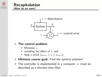
Recapitulation What do we want? v = disturbance y u System e = - PowerPoint PPT Presentation

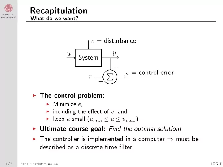
Recapitulation What do we want? v = disturbance y u System − e = control error r � + ◮ The control problem: ◮ Minimize e , ◮ including the effect of v , and ◮ keep u small ( u min ≤ u ≤ u max ). ◮ Ultimate course goal: Find the optimal solution! ◮ The controller is implemented in a computer ⇒ must be described as a discrete-time filter. 1 / 8 LQG 1 hans.rosth@it.uu.se

Recapitulation, cont’d What have we achieved? — summary of what we have looked at so far ◮ Discrete-time systems: ◮ Difference equations, ◮ shift operator q , ◮ stability region = inside of the unit circle. ◮ Sampling of systems = zero-order hold sampling (ZOH): ◮ Exact for t = kh , ◮ sampling period = h , ◮ Nyquist frequency ω n = ω s / 2 = π/h , ◮ frequency response of G ( z ) for z = e iωh . ◮ MIMO systems: Straightforward to use state space forms. ◮ Disturbance models: ◮ Spectral density: Φ( ω ) = F [ r ( τ )] , ◮ white noise v ⇔ Φ v ( ω ) = R v = const., ◮ linear filtering: y = Gu ⇒ Φ y = | G | 2 Φ u , ◮ spectral factorization: Φ = | G | 2 R , ◮ Lyapunov equation ⇒ Π x = Exx T . ◮ Kalman filters: Optimal observer, Riccati equations (CARE, DARE). 2 / 8 LQG 1 hans.rosth@it.uu.se

Control design Starting point in the continuous-time case ◮ Use the “standard” state space representation  x = Ax + Bu + Nv 1 , ˙ � R 1  � v 1 � � R 12  z = Mx, η = , Φ η ( ω ) = R T v 2 R 2 12  y = Cx + v 2 ,  ◮ Minimize the criterion z T Q 1 z + u T Q 2 u V = || z || 2 Q 1 + || u || 2 � � Q 2 = E ◮ The weighting matrices, Q 1 = Q T Q 2 = Q T 1 ≥ 0 and 2 > 0 , are design parameters. 3 / 8 LQG 1 hans.rosth@it.uu.se

Control strategy State feedback with observer The optimal controller is conveniently represented as state feedback from estimated states. ◮ Control law: u ( t ) = − L ˆ x ( t ) + ˜ r ( t ) ◮ Observer: ˙ x ( t ) = A ˆ ˆ x ( t ) + Bu ( t ) + K ( y ( t ) − C ˆ x ( t )) ◮ The control law can also be written as U ( s ) = F r ( s ) ˜  R ( s ) − F y ( s ) Y ( s ) ,   F y ( s ) = L ( sI − A + BL + KC ) − 1 K,  F r ( s ) = I − L ( sI − A + BL + KC ) − 1 B  ◮ The poles of the closed loop system are the roots of 0 = det( sI − A + BL ) · det( sI − A + KC ) , i.e. poles from state feedback + the observer poles. 4 / 8 LQG 1 hans.rosth@it.uu.se

LQG: The optimal controller Theorem 9.1 ◮ The optimal control law is u ( t ) = − L ˆ x ( t ) , ◮ ˆ x ( t ) is obtained from the corresponding Kalman filter . ◮ The optimal state feedback gain is 2 B T S, L = Q − 1 ◮ the matrix S = S T ≥ 0 is the solution to the continuous-time algebraic Riccati equation (CARE) 0 = A T S + SA + M T Q 1 M − SBQ − 1 2 B T S ◮ N.B. There are two different CAREs involved, the one above and the one for the Kalman filter! ◮ Some technical conditions: ( A, B ) stabilizable, ( A, C ) and ( A, M T Q 1 M ) detectable... 5 / 8 LQG 1 hans.rosth@it.uu.se

LQ/LQG: Properties ◮ A − BL is always stable ◮ The control law u = − Lx ( t ) (pure state feedback) is optimal, also for the deterministic case ( v 1 = 0 and v 2 = 0 ) ⇔ LQ = l inear q uadratic control. ◮ If v 1 and v 2 have Gaussian distributions the controller is the optimal controller (Cor. 9.1) ⇔ LQG = l inear q uadratic G aussian control. ◮ Theorem 9.1 = the separation theorem : The optimal observer = the Kalman filter, combined with the optimal state feedback (LQ) give the optimal controller! (This is far from obvious...) ◮ The LQ/LQG controller looks exactly the same for SISO and MIMO systems. 6 / 8 LQG 1 hans.rosth@it.uu.se

The servo problem How can the reference signal r ( t ) be included? ◮ General solution: Characterize r ( t ) by its spectrum and model it in the same way as a disturbance, i.e. incorporate it in the model. ◮ Special case, Theorem 9.2: If r ( t ) is piecewise constant, then the criterion V = || z − r || 2 Q 1 + || u − u ∗ ( r ) || 2 Q 2 is minimized with the control law u ( t ) = − L ˆ x ( t ) + L r r ( t ) , where L and ˆ x ( t ) are given as in Theorem 9.1, and L r is chosen so that I = M ( sI − A + BL ) − 1 BL r � s =0 = G c (0) L r . � (Then u ∗ ( r ) = L r r .) 7 / 8 LQG 1 hans.rosth@it.uu.se

Example: LQ control of a DC-motor The effect of Q 1 and Q 2 1 ◮ The DC-motor: Y ( s ) = s ( s +1) U ( s ) Design parameters: Q 1 = 1 , Q 2 = 1 / 0 . 1 / 0 . 01 LQ control ⇒ pure state feedback: u ( t ) = − Lx ( t ) + mr ( t ) ◮ Simulations: Step responses for the closed loop systems. ◮ The outputs, y : Q 2 = 1 Q 2 = 0 . 1 Q 2 = 0 . 01 ◮ The inputs, u : Q 2 = 0 . 01 Q 2 = 0 . 1 Q 2 = 1 8 / 8 LQG 1 hans.rosth@it.uu.se