reached with positive probability under behavior strategies i i - PDF document
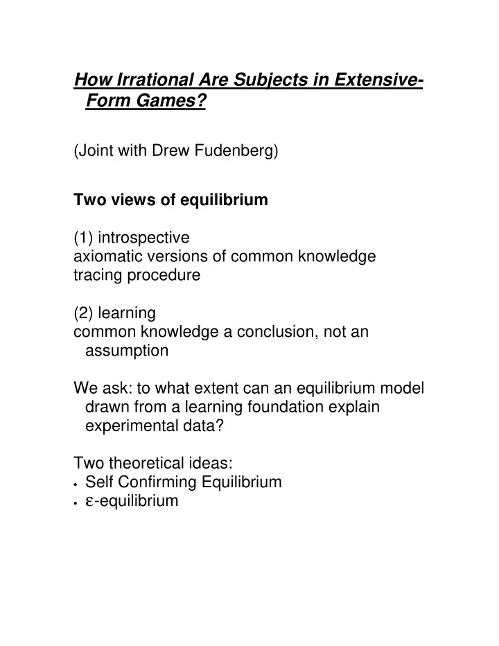
How Irrational Are Subjects in Extensive- Form Games? (Joint with Drew Fudenberg) Two views of equilibrium (1) introspective axiomatic versions of common knowledge tracing procedure (2) learning common knowledge a conclusion, not an
How Irrational Are Subjects in Extensive- Form Games? (Joint with Drew Fudenberg) Two views of equilibrium (1) introspective axiomatic versions of common knowledge tracing procedure (2) learning common knowledge a conclusion, not an assumption We ask: to what extent can an equilibrium model drawn from a learning foundation explain experimental data? Two theoretical ideas: • Self Confirming Equilibrium • ε -equilibrium
Two views of experiments (1) The stakes are too small to matter (extreme view of ε -equilibrium) (2) The results do not support the “theory” (usually means some refinement of Nash equilibrium) Many proponents of (2) use results to argue against rationality, at least in the narrow sense of maximizing monetary payoff 2
Self Confirming Equilibrium ∈ pure strategies for i; σ i ∈Σ mixed s S i i i H i information sets for i H ( ) σ reached with positive probability under σ ∈Π behavior strategies π i i � ( i map from mixed to behavior strategies ) π σ h i ρ π , � ( ) distribution over terminal � ( ) � ( � ( )) ρ σ ≡ ρ π σ nodes µ i a probability measure on Π − i ( ) µ preferences u s i i i ( ) { ( ) � ( ), } Π − σ ≡ π π = π σ ∀ ∈ ∩ J h h h H J − − − i i i i i i i i i 3
Nash equilibrium a mixed profile σ such that for each ∈ supp( ) σ there exist beliefs µ i such that s i i ( ) ⋅µ s i maximizes u i • i ( ( )) = 1 µ Π − σ i H − • i i Unitary Self-Confirming Equilibrium ( ( | ( ))) = 1 µ Π − σ σ i H − • i i (=Nash with two players) Heterogeneous Self-Confirming equilibrium ( ( | ( , ))) = 1 µ Π − σ σ H s − • i i i i Can summarize by means of “observation function” ( , ) , ( ), ( , ) σ = σ σ J s H H H s i i 4
Public Randomization (3,1) U L 1 R 2 (2,2) D (1,0) Remark: In games with perfect information, the set of heterogeneous self-confirming equilibrium payoffs (and the probability distributions over outcomes) are convex 5
to go beyond self-confirming in general requires experimentation might expect self-confirming in the medium run (Roth-Erev simulations; McKelvey-Palfrey estimation), and if enough experimentation Nash in the long-run another paper “Self-confirming Equilibrium” explores in detail the connection between self- confirming, correlated and Nash 6
Approximate Equilibrium exact: u s ( ) ( ) µ ≥ ′ µ u s • i i i i i i approximate: u s ( ) ( ) µ + ε ≥ ′ µ u s i i i i i i • Approximate equilibrium can be very different from exact equilibrium Radner’s work on finite repeated PD gang of four on reputation A small portion of the population playing "non- optimally" may significantly change the incentives for other players causing a large shift in equilibrium behavior. 7
How big is big? • we propose to measure how big is, that is to measure the minimal value of ε consistent with players’ play • given the observed distribution over terminal nodes we will “attribute” a loss to each terminal node and report the distribution of losses • somewhat involved procedure in general due to the fact that in extensive form games we do not directly observe players’ strategies • while the distribution we report has some arbitrary accounting conventions, such as attributing as much of the loss as possible to the final moves of the game, the mean loss is uniquely defined and independent of the particular accounting convention distribution over outcome is ρ loss attributed to z is ε ( , ( ), ) ⋅ ρ i z J mean ε ( ( ), ) ⋅ ρ i J 8
J ( ) ⋅ observation function for unitary or heterogeneous 9
Sample Calculation from Centipede Game P 1 P 2 P 3 P 4 1 2 1 2 ($6.40,$1.60) [0.92] [0.51] [0.25] [0.18] T 1 [0.08] T 2 [0.49] T 3 [0.75] T 4 [0.82] ($0.40,$0.10)($0.20,$0.80)($1.60,$0.40)($0.80,$3.20) ) “worst subsequent payoff” ( m a i i for player 1 P T 1 $0.20 $0.40 3 $0.80 $1.60 10
y probability distribution over payoffs p i y where y is a subgame 0 , , , P P P 1 2 3 for player 1 at P 3 (.18 $6.40, .82 $0.80) at y 2 for a , = i = P T P 3 3 ∑ ∑ ’ y ( , ) max{ ,max 0 ( ’ ) ( ) ( ’ )} ε ρ ≡ − π a m a up u y a ’ ( ) i a ∈ g y i i i ’ i y u i max ( ’ ) = 1 60 $ . m a ’ ( ) a ∈ g y i i i ’ ∑ ∑ y ( ) ( ’ ) $ . 1 60 π = up u y T 3 i ’ y u ∑ ∑ ’ y ( ) ( ’ π ) = . 18 ⋅ $ . 6 40 + . 82 ⋅ $ . 0 80 = $ . 1 808 up u y P 3 i ’ y u ( , ) 0 , ( , ) 0 ε ρ = ε ρ = T P 3 3 since ε = 0 , we assign the actual probabilities to the actual payoffs p P = ( . 0 75 1 60 0 25 18 6 40 82 0 80 $ , , . (. $ . ,. $ . )) 3 1 to understand algorithm, if ε > 0 for an action, then the probability of that action is assigned m i (player knows he could get at least this much) add up over actions to get terminal node losses 11
Centipede Game: Palfrey and McKelvey P 1 P 2 P 3 P 4 1 2 1 2 ($6.40,$1.60) [0.92] [0.51] [0.25] [0.18] T 1 [0.08] T 2 [0.49] T 3 [0.75] T 4 [0.82] ($0.40,$0.10)($0.20,$0.80)($1.60,$0.40)($0.80,$3.20) Numbers in square brackets correspond to the observed conditional probabilities of play corresponding to rounds 6-10, stakes 1x below. This game has a unique self-confirming equilibrium; in it player 1 with probability 1 plays T 1 12
Trials Rnds Stake Ca Expected Max Ratio / s Loss e Rnd Pl 1 Pl 2 Both Gain 29* 6-10 1x H $0.00 $0.03 $0.02 $4.0 0.4% 0 29* 6-10 1x U $0.26 $0.17 $0.22 $4.0 5.4% 0 WC 1x H $0.80 $4.0 20.0 0 % 29 1-10 1x H $0.00 $0.08 $0.04 $4.0 1.0% 0 10 1-10 4x H $0.00 $0.28 $0.14 $16. 0.9% 00 Rnds=Rounds, WC=Worst Case, H=Heterogeneous, U=Unitary *The data on which from which this case is computed is reported above. 13
• heterogeneous loss per player is small; because payoffs are doubling in each stage, equilibrium is very sensitive to a small number of player 2’s giving money away at the end of the game. • unknowing losses far greater than knowing losses • quadrupling the stakes very nearly causes ε to quadruple • theory has substantial predictive power: see WC • losses conditional on reaching the final stage are quite large--inconsistent with subgame perfection. McKelvey and Palfrey estimated an incomplete information model where some “types” of player 2 liked to pass in the final stage. This cannot explain many players dropping out early so their estimated model fits poorly. 14
Heterogeneous Losses Player 2 (H) 1.00 0.80 0.60 0.40 0.20 0.00 $0.00 $1.60 (No player 1 heterogeneous losses) 15
Unitary Losses Player 1 (U) 0.60 0.50 0.40 0.30 0.20 0.10 0.00 $0.00 $0.35 $0.62 $0.35 for dropping out in stage 3 $0.62 for dropping out in stage 1. Player 2 (U) 0.60 0.50 0.40 0.30 0.20 0.10 0.00 $0.00 $0.30 $1.60 $0.30 for dropping out in stage 2: expected loss of $0.14 $1.60 for giving away money at end: expected loss of $0.03 16
Best Shot Game: Prasnikar and Roth (W(max(x 1 ,x 2 )-C(x 1 ), 1 x 1 2 x 2 W(max(x 1 ,x 2 )-C(x 2 )) x W(x) C(x) 0 $0.00 $0.00 1 $1.00 $0.82 2 $1.95 $1.64 3 $2.85 $2.46 4 $3.70 $3.28 5 $4.50 $4.10 6 $5.25 $4.92 7 $5.95 $5.74 8 $6.60 $6.50 17
if the other player makes any contribution at all, it is optimal to contribute nothing unique subgame perfect equilibrium player 1 contributes nothing another Nash equilibrium player 2 to contributes nothing regardless of player 1’s play it is not consistent with Nash equilibrium for some player 1’s to play 0 and others 4 any other probability distribution over the two Nash equilibria are heterogeneous self- confirming 18
Trials Rnds Info Case Expected Loss Max Ratio Pl 1 Pl 2 Both Gain 8 8-10 full H $0.00 $0.12 $0.06 $2.06 2.9% 8 8-10 full U $0.00 $0.12 $0.06 $2.06 2.9% 10 8-10 part H $0.01 $0.15 $0.08 $2.06 3.9% 10 8-10 part U $0.39 $0.15 $0.27 $2.06 13.% WC H $3.41 $2.06 165% Rnds=Rounds, WC=Worst Case, H=Heterogeneous, U=Unitary 19
• In the full information case and partial information heterogeneous case player 2 occasionally contributes less than 4 when player 1 has contributed nothing; Note that the player who contributes nothing gets $3.70 against $0.42 for the opponent who contributes 4 • larger losses than centipede game with lower stakes • full information case heterogeneous losses equal unitary losses-- player 1 never contributed anything, and so never had a loss with either type of information; all losses by player 2 are necessarily knowing losses • In the partial information case occasionally player 1 contributed 4 and player 2 contributed nothing: looks like public randomization between the two Nash equilibria. This is inconsistent with Nash equilibrium but consistent with self-confirming equilibrium. 20
Partial Information Loss Distribution Player 2 Player 2 (H,U) 0.60 0.50 0.40 0.30 0.20 0.10 0.00 $0.00 $0.10 $0.20 $0.30 $0.40 $0.50 $0.60 losses correspond almost entirely to under contributing when player 1 has failed to contribute (in one case a player 2 wasted money by contributing when player has already contributed--it is hard to find much of a rationale for this, since neither player benefited by 2’s action) 21
Recommend
More recommend
Explore More Topics
Stay informed with curated content and fresh updates.
