Random variables DS GA 1002 Statistical and Mathematical Models - PowerPoint PPT Presentation

Example: Call center Pmf of binomial with parameters n and p = λ n converges to pmf of Poisson with parameter λ This is an example of convergence in distribution

Binomial random variable n = 40, p = 20 40 0 . 15 0 . 1 5 · 10 − 2 0 0 10 20 30 40 k

Binomial random variable n = 80, p = 20 80 0 . 15 0 . 1 5 · 10 − 2 0 0 10 20 30 40 k

Binomial random variable n = 400, p = 20 400 0 . 15 0 . 1 5 · 10 − 2 0 0 10 20 30 40 k

Poisson random variable λ = 20 0 . 15 0 . 1 5 · 10 − 2 0 0 10 20 30 40 k

Call-center data ◮ Assumptions do not hold over the whole day (why?) ◮ They do hold (approximately) for intervals of time ◮ Example: Data from a call center in Israel ◮ We compare the histogram of the number of calls received in an interval of 4 hours over 2 months and the pmf of a Poisson random variable fitted to the data

Call-center data 0.14 Real data 0.12 Poisson distribution 0.10 0.08 0.06 0.04 0.02 0.00 0 5 10 15 20 25 30 35 40 Number of calls

Discrete random variables Continuous random variables Conditioning on an event Functions of random variables

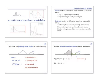
Continuous random variables Useful to model continuous quantities without discretizing Assigning nonzero probabilities to events of the form { X = x } for x ∈ R doesn’t work! Instead, we only consider events of the form { X ∈ S} where S is a union of intervals (formally a Borel set) We cannot consider every possible subset of R for technical reasons

Cumulative distribution function The cumulative distribution function (cdf) of X is defined as F X ( x ) := P ( { X ( ω ) ≤ x : ω ∈ Ω } ) = P ( X ≤ x ) In words, F X ( x ) is the probability of X being smaller than x The cdf can be defined for both continuous and discrete random variables

Cumulative distribution function The cdf completely specifies the distribution of the random variable The probability of any interval ( a , b ] is given by P ( a < X ≤ b ) = P ( X ≤ b ) − P ( X ≤ a ) = F X ( b ) − F X ( a ) To define a continuous random variable we just need a valid cdf! A valid underlying probability space exists, but we don’t need to worry about it

Properties of the cdf x →−∞ F X ( x ) = 0 , lim x →∞ F X ( x ) = 1 , lim F X ( b ) ≥ F X ( a ) if b > a , i.e. F X is nondecreasing

Probability density function When the cdf is differentiable, its derivative can be interpreted as a density Probability density function f X ( x ) := d F X ( x ) d x The pdf is not a probability measure! (It can be greater than 1)

Probability density function By the fundamental theorem of calculus P ( a < X ≤ b ) = F X ( b ) − F X ( a ) � b = f X ( x ) d x a Intuitively, ∆ → 0 P ( X ∈ ( x , x + ∆)) = f X ( x ) ∆ lim

Properties of the pdf For any union of intervals (any Borel set) S � P ( X ∈ S ) = f X ( x ) d x S In particular, � ∞ f X ( x ) d x = 1 −∞ From the monotonicity of the cdf f X ( x ) ≥ 0

Uniform random variable Pdf of a uniform random variable with domain [ a , b ] : � 1 b − a , if a ≤ x ≤ b , f X ( x ) = 0 , otherwise

Uniform random variable in [ a , b ] 1 b − a f X ( x ) 0 a b x

Exponential random variable Used to model waiting times (time until a certain event occurs) Examples: decay of a radioactive particle, telephone call, mechanical failure of a device Pdf of an exponential random variable with parameter λ : � λ e − λ x , if x ≥ 0 , f X ( x ) = 0 , otherwise

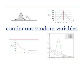
Exponential random variables λ = 0 . 5 1 . 5 λ = 1 . 0 λ = 1 . 5 1 f X ( x ) 0 . 5 0 0 2 4 6 8 x

Call-center data ◮ Example: Data from a call center in Israel ◮ We compare the histogram of the inter-arrival times between calls occurring between 8 pm and midnight over two days and the pdf of an exponential random variable fitted to the data

Call center 0.9 Exponential distribution 0.8 Real data 0.7 0.6 0.5 0.4 0.3 0.2 0.1 0.0 0 1 2 3 4 5 6 7 8 9 Interarrival times (s)

Gaussian or normal random variable Extremely popular in probabilistic models and statistics Sums of independent random variables converge to Gaussian distributions under certain assumptions Pdf of a Gaussian random variable with mean µ and standard deviation σ e − ( x − µ ) 2 1 f X ( x ) = √ 2 σ 2 2 πσ

Gaussian random variables µ = 2 σ = 1 0 . 4 µ = 0 σ = 2 µ = 0 σ = 4 0 . 3 f X ( x ) 0 . 2 0 . 1 0 − 10 − 5 0 5 10 x

Height data ◮ Example: Data from a population of 25 000 people ◮ We compare the histogram of the heights and the pdf of a Gaussian random variable fitted to the data

Height data 0.25 Gaussian distribution Real data 0.20 0.15 0.10 0.05 60 62 64 66 68 70 72 74 76 Height (inches)

Problem ◮ The Gaussian cdf does not have a closed form solution ◮ This complicates computing the probability that a Gaussian belongs to a set

Standard Gaussian If X is Gaussian with mean µ and standard deviation σ , then U := X − µ σ is a standard Gaussian, with mean zero and unit standard deviation � X − µ � a − µ �� , b − µ P ( X ∈ [ a , b ]) = P ∈ σ σ σ � b − µ � � a − µ � = Φ − Φ σ σ Φ is the cdf of a standard Gaussian, which is tabulated

χ 2 random variable Very important in hypothesis testing If U 1 , U 2 , . . . , U d are d independent standard Gaussian random variables d � U 2 X := i i = 1 is a χ 2 with d degrees of freedom

χ 2 random variable The pdf of a χ 2 random variable with d degrees of freedom is 2 − 1 exp d � − x � f X ( x ) = x 2 � d d 2 Γ � 2 2 if x > 0 and zero otherwise

χ 2 random variables 0 . 5 d = 1 d = 5 0 . 4 d = 10 0 . 3 f X ( x ) 0 . 2 0 . 1 0 0 5 10 15 20 25 x

Discrete random variables Continuous random variables Conditioning on an event Functions of random variables

Conditioning on an event We usually define random variables using their pmf, cdf or pdf How can we incorporate the information that X ∈ S for some set S ?

Conditional pmf If X has pmf p X , the conditional pmf of X given X ∈ S is p X | X ∈S ( x ) := P ( X = x | X ∈ S ) p X ( x ) � if x ∈ S � s ∈S p X ( s ) = 0 otherwise . Valid pmf in the new probability space restricted to the event { X ∈ S}

Conditional cdf If X has pdf f X , the conditional cdf of X given X ∈ S is F X | X ∈S ( x ) := P ( X ≤ x | X ∈ S ) = P ( X ≤ x , X ∈ S ) P ( X ∈ S ) � u ≤ x , u ∈S f X ( u ) d u = � u ∈S f X ( u ) d u Valid cdf in the new probability space restricted to the event { X ∈ S}

Example: Geometric random variables are memoryless We flip a coin repeatedly until we obtain heads, but pause after k 0 flips (which were tails) What is the probability of obtaining heads in k more flips?

Example: Geometric random variables are memoryless P ( k more flips )

Example: Geometric random variables are memoryless P ( k more flips ) = p X | X > k 0 ( k )

Example: Geometric random variables are memoryless P ( k more flips ) = p X | X > k 0 ( k ) p X ( k ) = � ∞ m = k 0 + 1 p X ( m )

Example: Geometric random variables are memoryless P ( k more flips ) = p X | X > k 0 ( k ) p X ( k ) = � ∞ m = k 0 + 1 p X ( m ) ( 1 − p ) k − 1 p = m = k 0 + 1 ( 1 − p ) m − 1 p � ∞

Example: Geometric random variables are memoryless P ( k more flips ) = p X | X > k 0 ( k ) p X ( k ) = � ∞ m = k 0 + 1 p X ( m ) ( 1 − p ) k − 1 p = m = k 0 + 1 ( 1 − p ) m − 1 p � ∞ = ( 1 − p ) k − k 0 − 1 p for k > k 0 Geometric series: ∞ α k 0 α m − 1 = � for any α < 1 1 − α m = k 0 + 1

Example: Exponential random variables are memoryless Assume email inter-arrival times are exponential with parameter λ You get an email, then no email for t 0 minutes How is the waiting time until the next email distributed now?

Example: Exponential random variables are memoryless F T | T > t 0 ( t )

Example: Exponential random variables are memoryless � t t 0 f T ( u ) d u F T | T > t 0 ( t ) = � ∞ t 0 f T ( u ) d u

Example: Exponential random variables are memoryless � t t 0 f T ( u ) d u F T | T > t 0 ( t ) = � ∞ t 0 f T ( u ) d u = e − λ t − e − λ t 0 − e − λ t 0

Example: Exponential random variables are memoryless � t t 0 f T ( u ) d u F T | T > t 0 ( t ) = � ∞ t 0 f T ( u ) d u = e − λ t − e − λ t 0 − e − λ t 0 = 1 − e − λ ( t − t 0 ) for t > t 0

Example: Exponential random variables are memoryless � t t 0 f T ( u ) d u F T | T > t 0 ( t ) = � ∞ t 0 f T ( u ) d u = e − λ t − e − λ t 0 − e − λ t 0 = 1 − e − λ ( t − t 0 ) for t > t 0 Differentiating with respect to t f T | T > t 0 ( t ) = λ e − λ ( t − t 0 ) for t > t 0

Discrete random variables Continuous random variables Conditioning on an event Functions of random variables

Functions of random variables ◮ For any deterministic function g and r.v. X , Y := g ( X ) is a random variable ◮ Formally, X maps elements of Ω to R , so Y does too since Y ( ω ) = g ( X ( ω ))

Discrete random variables If X is discrete p Y ( y ) = P ( Y = y ) = P ( g ( X ) = y ) � = p X ( x ) { x | g ( x )= y }