Random Variables, Distributions, and Moments IE 502: Probabilistic - PowerPoint PPT Presentation

Random Variables, Distributions, and Moments IE 502: Probabilistic Models Jayendran Venkateswaran IE & OR

Example: ‘Continuum’ • Suppose a student has a class at 9.30am. The student, as usual leaves his hostel in the last minute. He is likely to be late but will definitely reach the class before 10.30am. How likely is it that student is delayed by no more than 30 mins? • Outcome Random variable • Wall Clock Time delay time, X, [0, 1] hour • To obtain probabilities, let’s assume an auxiliary function, f , to be −2 x + 2 for x in [0, 1] IE502: Probabilistic Models IEOR @ IITBombay

Continuous r.v. – density function • Continuous r.v.  whose set of possible values are uncountable. – Makes definition of pdf more cumbersome than pmf • Probability density function (pdf) assigns a probability density to each and every value of r.v. • Example: ‘Continuum’ Delay IE502: Probabilistic Models IEOR @ IITBombay

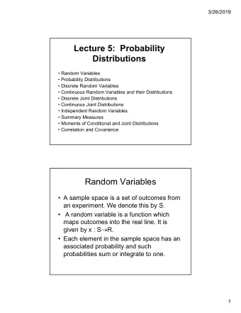
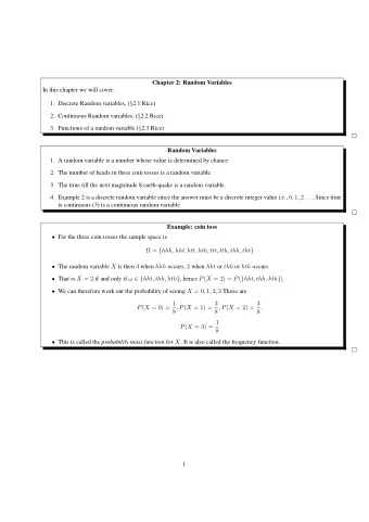
Summary • Random variables – Defining r.v: Discrete and continuous – Outcomes, random variables, and events • Cumulative distribution function (cdf): F(x) • Discrete r.v. – Probability mass function (pmf): p(x) • Continuous random variable – Probability density function (pdf): f(x) IE502: Probabilistic Models IEOR @ IITBombay

Expectation of random variable • Expectation or Expected Value or Mean 1. If X is a discrete r.v. with pmf p ( x ), then expected value of X is … • Three coin toss example 1. If X is a continuous r.v. with pdf f ( x ), then expected value of X is … – Delay example IE502: Probabilistic Models IEOR @ IITBombay

Expectation of a Function of a r.v. • We are interested in the expected value of some function of r.v. X , say, g ( X ) • Proposition 2.1 – If X is a discrete random variable with pmf p ( x ), then for any real-values function g , ∑ = E [ g ( X )] g ( x ) p ( x ) x – If X is a continuous random variable with pdf f ( x ), then for any real-values function g , ∞ ∫ = E [ g ( X )] g ( x ) f ( x ) dx − ∞ IE502: Probabilistic Models IEOR @ IITBombay

Moments of a random variable • The n th moment of r.v. X is E[ X n ], n ≥1 – 1 st moment is the mean • The n th central moment of r.v. X is E[ ( X − E[ X ]) n ] – First central moment is 0 – Second central moment is Variance, the amount of variability in the values of the r.v. – Positive square root of variance is standard deviation σ • Compute Var(X) – Three coin toss example – Student delay example IE502: Probabilistic Models IEOR @ IITBombay

Central Moments • Normalized moments – Normalized n th moment is the n th central moment divided by σ n • Third central moment – Measures lopsidedness of the distribution – Skewness  normalized third central moment – Skewness = 0 for symmetric distributions Positive skew Negative skew IE502: Probabilistic Models IEOR @ IITBombay

Central moment (contd) • Fourth Central Moment – Measure of whether distribution is measure of “peakedness” – distribution is tall and skinny or short and squat (compared to the Normal distribution) – Kurtosis  normalized fourth central moment − 3 IE502: Probabilistic Models IEOR @ IITBombay

Theoretical Distributions IE 502: Probabilistic Models Jayendran Venkateswaran IE & OR

Introduction • Theoretical distributions have been derived based on certain facts/ principles/ assumptions by logical or mathematical reasoning – Allows us to make rational judgments concerning probability of events IE502: Probabilistic Models IEOR @ IITBombay

Discrete Probability Distributions IE502: Probabilistic Models IEOR @ IITBombay

Bernoulli Distribution • Named after James Bernoulli – Bernoulli trials • X ~ Bernoulli( p ) • X takes on value 1 with success probability p and value 0 with failure probability q =1- p • PMF Bernoulli trial is an experiment whose outcome is random & can be either of 2 • Expected Value & Variance possible outcomes, "success" & "failure" IE502: Probabilistic Models IEOR @ IITBombay

Binomial Distribution • Has foundation in Bernoulli trials/process • X ~ Binomial( n , p ) • X is the number of successes in n trials, where each trial can result in success with probability p and failure with probability q = 1- p • PMF • Expected Value & Variance IE502: Probabilistic Models IEOR @ IITBombay

Bernoulli trials & Binomial Distribution IE502: Probabilistic Models IEOR @ IITBombay

Binomial Distribution - pmf p=0.5, n =10 p=0.5, n =20 p=0.7, n =20 IE502: Probabilistic Models IEOR @ IITBombay

Geometric Distribution • Has foundation in the Bernoulli trials/process • X ~ Geometric( p ) • X is the number of trials required until the first success, where each trial can result in success with probability p • PMF • Expected Value & Variance IE502: Probabilistic Models IEOR @ IITBombay