The Normal Distribution August 8, 2019 August 8, 2019 1 / 80 - PowerPoint PPT Presentation

The Normal Distribution August 8, 2019 August 8, 2019 1 / 80

Distributions of Random Variables We’ve spent the past week talking about random variables. We’ve also talked about probability distributions. In Chapter 4, we are going to put these two concepts together to think about some common distributions that we use to model random variables. Section 4.1 August 8, 2019 2 / 80

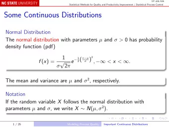
The Normal Distribution We start our discussion with the normal distribution . This is one of the most common distributions you will see in practice. Section 4.1 August 8, 2019 3 / 80

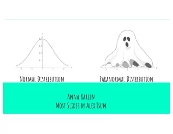
The Normal Distribution Normal distributions are always... Symmetric. Unimodal. ”Bell curves”. Variables such as SAT scores closely follow the normal distribution. Section 4.1 August 8, 2019 4 / 80

The Normal Distribution The normal distribution has most measurements falling somewhere near the middle - or average - and values get less and less likely as we move further into the tails. Variables such as SAT scores closely follow the normal distribution. Section 4.1 August 8, 2019 5 / 80

Normal Distributions Many variables are nearly normal, but none are exactly normal. While not perfect for any single problem, the normal distribution is very useful for a variety of problems. We will use it in data exploration and to solve important problems in statistics. Section 4.1 August 8, 2019 6 / 80

The Normal Distribution Model The symmetric, unimodal, bell-shaped curve of the normal distribution can vary based on: Mean Standard deviation These adjustable details are called model parameters . Section 4.1 August 8, 2019 7 / 80

Parameters: Normal Distribution Changing the mean shifts the curve to the left or right. Changing the standard deviation stretches or constricts the curve. (This can make the peak appear narrower or flatter.) Section 4.1 August 8, 2019 8 / 80

Parameters: Normal Distribution The distribution on the left has µ = 0 and σ = 1. The distribution on the right has µ = 19 and σ = 4 These look exactly the same because the scale of the axis has been adjusted. Section 4.1 August 8, 2019 9 / 80

Parameters: Normal Distribution These are the same two distributions, now on the same axis. Now we can see that the shift of the mean from 0 to 19 moves the distribution to the right. The change in standard deviation from 1 to 4 flattens the distribution. Section 4.1 August 8, 2019 10 / 80

Normal Distribution Notation For a normal distribution with mean µ and standard deviation σ , we write N ( µ, σ ) For a variable X with a normal distribution, we may write X ∼ N ( µ, σ ) . where ” ∼ ” denotes ”is distributed”. Section 4.1 August 8, 2019 11 / 80

Normal Distribution Notation For a normal distribution with mean 19 and standard deviation 4, we write N ( µ = 19 , σ = 4) The mean and standard deviation describe a normal distribution fully and exactly. This is what we mean by a distribution’s parameters . Section 4.1 August 8, 2019 12 / 80

Standard Normal Distribution The standard normal distribution is a normal distribution with mean µ = 0 and standard deviation σ = 1. N ( µ = 0 , σ = 1) Section 4.1 August 8, 2019 13 / 80

Standardizing with Z-Scores We often want to put data onto a standardized scale, which can make comparisons more reasonable. Section 4.1 August 8, 2019 14 / 80

Example: SAT and ACT The distribution of SAT and ACT scores are both nearly normal. The table shows the mean and standard deviation for total scores on each. SAT ACT Mean 1100 21 SD 200 6 Suppose Ann scored 1300 on her SAT and Tom scored 24 on his ACT. Who performed better? Section 4.1 August 8, 2019 15 / 80

Example: SAT and ACT We can use the standard deviation to help us figure out who performed better. Ann’s SAT score is 1 standard deviation above average. 1100 + 200 = 1300 Tom’s ACT score is 0.5 standard deviations above average. 21 + 0 . 5 × 6 = 24 If you remember taking either test and being told your percentile, that’s the same idea! Section 4.1 August 8, 2019 16 / 80

Example: SAT and ACT We can also plot the normal distributions with scaled axes: Now we can see that Ann tends to do better with respect to everyone else than Tom does, so her score is better. Section 4.1 August 8, 2019 17 / 80

Standardizing with Z-Scores Our example got at a standardization technique called a Z-score. This method is commonly employed with normal distributions, but could also be used more generally. The Z-score of an observation is defined as the number of standard deviations it falls above or below the mean. If the observation is one standard deviation above the mean, its Z-score is 1. If it is 1.5 standard deviations below the mean, then its Z-score is -1.5. Section 4.1 August 8, 2019 18 / 80

Standardizing with Z-Scores We compute the Z-score for an observation x that follows a distribution with mean µ and standard deviation σ using z = x − µ σ Section 4.1 August 8, 2019 19 / 80

Example: Standardizing with Z-Scores The SATs had a mean score of µ SAT = 1100 and a standard deviation of σ SAT = 200. For Ann’s SAT score of 1300, the Z-score is z Ann = x Ann − µ SAT = 1300 − 1100 = 1 200 σ SAT Section 4.1 August 8, 2019 20 / 80

Example: Standardizing with Z-Scores The ACTs has mean µ = 21 and standard deviation σ = 6. Use Tom’s ACT score, 24, to find his Z-score. Section 4.1 August 8, 2019 21 / 80

Z-Scores Observations above the mean always have positive Z-scores. Observations below the mean always have negative Z-scores. If an observation is equal to the mean, the Z-score is always 0. Section 4.1 August 8, 2019 22 / 80

Example Let X represent a random variable from N ( µ = 3 , σ = 2) X ∼ N ( µ = 3 , σ = 2) and suppose we observe x = 5 . 19. 1 Find the Z-score of x. 2 Use the Z-score to determine how many standard deviations above or below the mean x falls. Section 4.1 August 8, 2019 23 / 80

Example We know from the problem statement that µ = 3, σ = 2, and our observed value is x = 5 . 19. So z = x − µ σ = 5 . 19 − 3 2 = 1 . 095 . Section 4.1 August 8, 2019 24 / 80

Example Using our definition of a Z-score, z = 1 . 095 means that the observations x is 1 . 095 standard deviations above the mean. We know that x is above the mean because the Z-score is positive. Section 4.1 August 8, 2019 25 / 80

Example: Brushtail Possums Head lengths of brushtail possums follow a normal distribution with mean 92.6 mm and standard deviation 3.6 mm. Compute the Z-scores for possums with head lengths of 95.4 mm and 85.8 mm. Section 4.1 August 8, 2019 26 / 80

Example: Brushtail Possums Let Y be the head lengths of brushtail possums. We say that Y ∼ N ( µ = 92 . 6 , σ = 3 . 6). For a head length of 95.4 mm, the Z-score will be z = y − µ σ = 95 . 4 − 92 . 6 3 . 6 = 0 . 78 . Section 4.1 August 8, 2019 27 / 80

Example: Brushtail Possums Let Y be the head lengths of brushtail possums. We say that Y ∼ N ( µ = 92 . 6 , σ = 3 . 6). For a head length of 85.8 mm, the Z-score will be z = y − µ σ = 85 . 8 − 92 . 6 3 . 6 = − 1 . 89 . Section 4.1 August 8, 2019 28 / 80

Example: Brushtail Possums The possum with a head length of 95.4 mm is 0.78 standard deviations above the mean ( z = 0 . 78). The possum with a head length of 85.8 mm is 1.89 standard deviations below the mean ( z = − 1 . 89). Section 4.1 August 8, 2019 29 / 80

Z-Scores and Unusual Observations We can use Z-scores to identify potentially unusual observations. An observation x 1 is more unusual than another observation x 2 is further from the mean. If z 1 and z 2 are the corresponding Z-scores, x 1 is more unusual than x 2 if | z 1 | > | z 2 | This technique is especially useful for symmetric distributions. Section 4.1 August 8, 2019 30 / 80

Example: Brushtail Possums We decided that The possum with a head length of 95.4 mm is 0.78 standard deviations above the mean ( z = 0 . 78). The possum with a head length of 85.8 mm is 1.89 standard deviations below the mean ( z = − 1 . 89). Since | − 1 . 89 | > | 0 . 78 | , we say the possum with the head length of 85.8 mm is more unusual than the other possum. Section 4.1 August 8, 2019 31 / 80

Finding Tail Areas Yesterday, we talked about using the area under a curve to think about proportions. Determining the area under the tail of a distribution is very useful in statistics! For example, your SAT percentile is the fraction of people who scored lower than you. Section 4.1 August 8, 2019 32 / 80

Finding Tail Areas We can visualize a tail area as the curve and shading shown. This is the distribution for SAT scores with Ann’s score as the cutoff point, at x = 1300. The area to the left of x is the percentile. Section 4.1 August 8, 2019 33 / 80

Finding Tail Areas There are several techniques for finding tail areas: 1 Integrate. 2 Use a graphing calculator. 3 Use a probability table. 4 Use a statistical software. Section 4.1 August 8, 2019 34 / 80

Finding Tail Areas: Integration The function that creates our normal distribution curve is 2 πσ 2 e − ( x − µ )2 1 f ( x ) = √ 2 σ 2 Don’t write this down. We won’t use it. In fact, it’s impossible to integrate this by hand! Section 4.1 August 8, 2019 35 / 80