Gov 2000: 2. Random Variables and Probability Distributions - PowerPoint PPT Presentation

Gov 2000: 2. Random Variables and Probability Distributions Matthew Blackwell Fall 2016 1 / 56

1. Random Variables 2. Probability Distributions 3. Cumulative Distribution Functions 4. Properties of Distributions 5. Famous distributions 6. Simulating Random Variables* 7. Wrap-up 2 / 56

Where are we going? variable. 3 / 56 Obama Presidential Approval (ANES 2016) 600 500 400 300 200 100 0 X = 0 X = 1 (Don't Approve) (Approve) • Long-term goal: inferring the data generating process of this ▶ What is the true Obama approval rate in the US? • Today: given a probability distribution, what data is likely? ▶ If we knew the true Obama approval, what samples are likely?

1/ Random Variables 4 / 56

Brief probability review probability: happen. ones are more likely than others. ℙ(𝐼𝐼) = ℙ(𝐼)ℙ(𝐼) = 0.5 × 0.5 = 0.25 5 / 56 • Ω is the sample space (set of events that could occur) • 𝜕 is a particular member of the sample space • Formalize uncertainty over which outcome will occur with ▶ ⇝ ℙ(𝜕) is the probability that a particular outcome will ▶ We don’t know which outcome will occur, but we know which • Example: tossing a fair coin twice ▶ Ω = {𝐼𝐼, 𝐼𝑈, 𝑈𝐼, 𝑈𝑈} ▶ Fair coins, independent,

What are random variables? Random Variable A random variable (r.v.) is a function that maps from the sample space of an experiment to the real line or 𝑌 ∶ Ω → ℝ . use math! 𝑌(𝜕) . 6 / 56 • r.v.s are numeric representation of uncertain events ⇝ we can • Lower-case letters 𝑦 are arbitrary values of the r.v. • Often 𝜕 is implicit and we just write the r.v. as 𝑌 instead of

Examples 𝑌 = 0 if don’t approve 1 if approve ⎩ { ⎨ { ⎧ variable because it’s not numeric. 7 / 56 • Tossing a coin 5 times ▶ one possible outcome: 𝜕 = 𝐼𝑈𝐼𝑈𝑈 , but not a random ▶ 𝑌(𝜕) = number of heads in the fjve tosses ▶ 𝑌(𝐼𝑈𝐼𝑈𝑈) = 2 • Obama approval for a respondent: ▶ Ω = { approve , don’t approve } . ▶ Random variable converts this into a number: ▶ Called a Bernoulli, binary, or dummy random variable. • Length of government in a parliamentary system: ▶ Ω = [0, ∞) ⇝ already numeric so 𝑌(𝜕) = 𝜕 .

2/ Probability Distributions 8 / 56

Randomness and probability all of the possible values of the r.v. distributions 9 / 56 • How are r.v.s random? ▶ Uncertainty over Ω ⇝ uncertainty over value of 𝑌 . ▶ We’ll use probability to formalize this uncertainty. • The probability distribution of a r.v. gives the probability of 0.6 0.5 More Likely 0.4 0.3 0.2 Less Likely Less Likely 0.1 0.0 -4 -2 0 2 4 x

Where do the probability distributions come from? data came to be. etc. DGP and a r.v. 10 / 56 • Probabilities on Ω induce probabilities for 𝑌 ▶ Independent fair coin fmips so that ℙ(𝐼) = 0.5 ▶ Then if 𝑌 = 1 for heads, ℙ(𝑌 = 1) = 0.5 • Data generating process (DGP): assumptions about how the ▶ Examples: coin fmips, randomly selecting a card from a deck, ▶ These assumptions imply probabilities over outcomes. ▶ Often we’ll skip the defjnition of Ω and directly connect the • Goal of statistics is often to learn about the distribution of 𝑌 .

Inducing probabilities 1/4 HT 1/4 1 TH 1/4 1 HH 2 1/4 𝑦 ℙ(𝑌 = 𝑦) 0 1/4 1 1/2 2 1/4 0 TT Ω | TT HT TH HH | 0 | 1 2 𝑌(𝜕) ℝ 1/4 1/4 1/4 1/4 𝜕 ℙ({𝜕}) 11 / 56 • Let 𝑌 be the number of heads in two coin fmips.

Probability mass function Discrete Random Variable confmict, number of parties elected to a legislature. 𝑔 𝑌 (𝑦) 𝑦∈𝑇 ℙ(𝑌 ∈ 𝑇) = ∑ 𝑔 𝑌 (𝑦 𝑘 ) = 1 𝑘=1 ∑ 𝑙 0 ≤ 𝑔 𝑌 (𝑦) ≤ 1 𝑔 𝑌 (𝑦) = ℙ(𝑌 = 𝑦) of 𝑌 when it is discrete: fjnite ( 𝑌 ∈ {𝑦 1 , … , 𝑦 𝑙 } ) or countably infjnite ( 𝑌 ∈ {𝑦 1 , 𝑦 2 , …} ). A r.v., 𝑌 , is discrete if its range (the set of values it can take) is 12 / 56 • Probability mass function (p.m.f.) describes the distribution • Some properties of the p.m.f. (from probability): • Probability of a set of values 𝑇 ⊂ {𝑦 1 , … , 𝑦 𝑙 } : • Examples: Obama approval, number of battle deaths in a

Example - random assignment to { 8 if (𝑈, 𝑈, 𝑈) 3 if (𝑈, 𝑈, 𝐷) or (𝐷, 𝑈, 𝑈) or (𝑈, 𝐷, 𝑈) 2 if (𝑈, 𝐷, 𝐷) or (𝐷, 𝑈, 𝐷) or (𝐷, 𝐷, 𝑈) 1 if (𝐷, 𝐷, 𝐷) 0 treatment { ⎩ { ⎧ ⎨ 𝑌 = 13 / 56 { { { • You want to run a randomized control trial on 3 people. • Use the following procedure: ▶ Flip independent fair coins for each unit ▶ Heads assigned to Control (C), tails to Treatment (T) • Let 𝑌 be the number of treated units: • Use independence and fair coins: ℙ(𝐷, 𝑈, 𝐷) = ℙ(𝐷)ℙ(𝑈)ℙ(𝐷) = 1 2 ⋅ 1 2 ⋅ 1 2 = 1

Calculating the p.m.f. 8 8 8 8 0! 14 / 56 𝑔 𝑌 (0) = ℙ(𝑌 = 0) = ℙ(𝐷, 𝐷, 𝐷) = 1 𝑔 𝑌 (1) = ℙ(𝑌 = 1) = ℙ(𝑈, 𝐷, 𝐷) + ℙ(𝐷, 𝑈, 𝐷) + ℙ(𝐷, 𝐷, 𝑈) = 3 𝑔 𝑌 (2) = ℙ(𝑌 = 2) = ℙ(𝑈, 𝑈, 𝐷) + ℙ(𝐷, 𝑈, 𝑈) + ℙ(𝑈, 𝐷, 𝑈) = 3 𝑔 𝑌 (3) = ℙ(𝑌 = 3) = ℙ(𝑈, 𝑈, 𝑈) = 1 • What’s ℙ(𝑌 = 4) ?

Plotuing the p.m.f. treatment? What is one major problem with it? 15 / 56 • We could plot this p.m.f. using R: 0.5 0.4 0.3 f(x) 0.2 0.1 0.0 0 1 2 3 x • Question : Does this seem like a good way to assign

Real-valued r.v.s subset of the real line? number. 0.232879873 … 0.57263048743 … 0.9823612984 … 16 / 56 • What if 𝑌 can take any value on ℝ or an uncountably infjnite • Can we just specify ℙ(𝑌 = 𝑦) ? • No! Proof by counterexample: ▶ Suppose ℙ(𝑌 = 𝑦) = 𝜁 for 𝑦 ∈ (0, 1) where 𝜁 is a very small ▶ What’s the probability of being between 0 and 1? ▶ There are an infjnite number of real numbers between 0 and 1: ▶ Each one has probability 𝜁 ⇝ ℙ(𝑌 ∈ (0, 1)) = ∞ × 𝜁 = ∞ • But ℙ(𝑌 ∈ (0, 1)) must be less than 1! • ⇝ ℙ(𝑌 = 𝑦) must be 0.

Thought experiment: draw a random real value between 0 and 10. 5982534904 2875546873 1159562863 8823537875 9375195778 2249534301 4654958537 1050792279 6892589235 4201995611 2129021960 8640344181 5981362977 4771309960 5187072113 4999999837 2978049951 0597317328 1609631859 5024459455 3469083026 4252230825 3344685035 2619311881 7101000313 7838752886 5875332083 8142061717 7669147303 1857780532 0005681271 4526356082 7785771342 7577896091 7363717872 1712268066 1300192787 6611195909 2164201989 3809525720 1065485863 2788659361 5338182796 8230301952 0353018529 6899577362 2599413891 2497217752 8347913151 5574857242 4541506959 5082953311 6861727855 8890750983 8175463746 4939319255 0604009277 0167113900 9848824012 8583616035 6370766010 4710181942 9555961989 4676783744... 1468440901 6094370277 0539217176 2931767523 8467481846 7669405132 What’s the probability that we draw a value that is exact equal to 4428810975 6659334461 2847564823 3786783165 𝜌 ? 3.1415926535 8979323846 2643383279 5028841971 6939937510 5820974944 5923078164 0628620899 8628034825 3421170679 8214808651 3282306647 0938446095 5058223172 5359408128 4811174502 8410270193 8521105559 6446229489 5493038196 2712019091 1907021798 4564856692 3460348610 4543266482 1339360726 0249141273 7245870066 0631558817 4881520920 9628292540 9171536436 7892590360 0113305305 4882046652 1384146951 9415116094 3305727036 5759591953 0921861173 8193261179 3105118548 0744623799 6274956735 1885752724 8912279381 8301194912 9833673362 4406566430 8602139494 6395224737 17 / 56

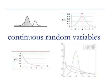
Probability density functions ℙ(𝑏 < 𝑌 < 𝑐) = ∫ governmental budgets allocations parliamentary system, proportion of voters who turned out, that region. Continuous Random Variable 𝑐 ℙ(𝑌 ∈ 𝐶) = ∫ interval, 𝐶 : A r.v., 𝑌 , is continuous if there exists a nonnegative function on ℝ , 18 / 56 𝑔 𝑌 called the probability density function (p.d.f.) such that for any 𝐶 𝑔 𝑌 (𝑦)𝑒𝑦 • Specifjcally, for a subset of the real line (𝑏, 𝑐) : 𝑏 𝑔 𝑌 (𝑦)𝑒𝑦. • ⇝ the probability of a region is the area under the p.d.f. for • Probability of a point mass: ℙ(𝑌 = 𝑑) = ∫ 𝑑 𝑑 𝑔 𝑌 (𝑦)𝑒𝑦 = 0 • Examples: length of time between two governments in a

The p.d.f. 𝑔 𝑌 (𝑦) ≠ ℙ(𝑌 = 𝑦) particular region. 19 / 56 0.6 0.5 0.4 f(x) 0.3 P ( 0 < X < 2 ) 0.2 0.1 0.0 -4 -2 0 2 4 x • The height of the curve is not the probability of 𝑦 : • We can use the integral to get the probability of falling in a

3/ Cumulative Distribution Functions 20 / 56

Cumulative distribution functions doesn’t depend on discrete vs. continuous: Cumulative distribution function The cumulative distribution function (c.d.f.) returns the probability is that a variable is less than a particular value: 𝐺 𝑌 (𝑦) ≡ ℙ(𝑌 ≤ 𝑦). like 𝑌 = 𝑦 ) on the real line. 21 / 56 • Useful to have a defjnition of the probability distribution that • Identifjes the probability of any interval (including singletons • For discrete r.v.: 𝐺 𝑌 (𝑦) = ∑ 𝑦 𝑘 ≤𝑦 𝑔 𝑌 (𝑦 𝑘 ) • For continuous r.v.: 𝐺 𝑌 (𝑦) = ∫ 𝑦 −∞ 𝑔 𝑌 (𝑢)𝑒𝑢