[PDF] - Probability and Random Processes Lecture 5 Probability and random PDF Document

SLIDE 1

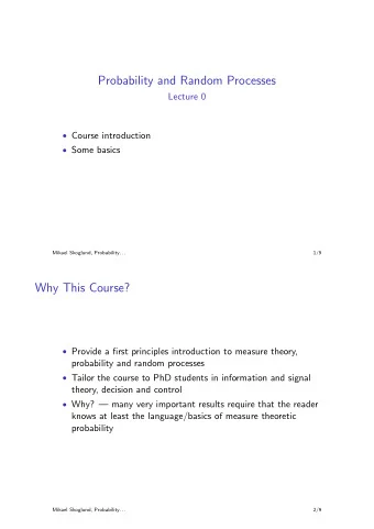
Probability and Random Processes

Lecture 5

Probability and random variables
The law of large numbers

Mikael Skoglund, Probability and random processes 1/21

Why Measure Theoretic Probability?

Stronger limit theorems
Conditional probability/expectation
Proper theory for continuous and mixed random variables

Mikael Skoglund, Probability and random processes 2/21

SLIDE 2

Probability Space

A probability space is a measure space (Ω, A, P)
the sample space Ω is the ’universe,’ i.e. the set of all possible
utcomes
the event class A is a σ-algebra of measurable sets called

events

the probability measure is a measure on events in A with the

property P(Ω) = 1

Mikael Skoglund, Probability and random processes 3/21

Interpretation

A random experiment generates an outcome ω ∈ Ω
For each A ∈ A either ω ∈ A or ω /

∈ A

An event A in A occurs if ω ∈ A with probability P(A)
since A is the σ-algebra of measurable sets, we are ensured

that all ’reasonable’ combinations of events and sequences of events are measurable, i.e., have probabilities

Mikael Skoglund, Probability and random processes 4/21

SLIDE 3

With Probability One

An event E ∈ A occurs with probability one if P(E) = 1
almost everywhere, almost certainly, almost surely,. . .

Mikael Skoglund, Probability and random processes 5/21

Independence

E and F in A are independent if P(E ∩ F) = P(E)P(F)
The events in a collection A1, . . . , An are
pairwise independent if Ai and Aj are independent for i = j
mutually independent if for any {i1, i2, . . . , ik} ⊆ {1, 2, . . . , n}

P(Ai1 ∩ Ai2 ∩ · · · ∩ Aik) = P(Ai1)P(Ai2) · · · P(Aik)

An infinite collection is mutually independent if any finite

subset of events is mutually independent

’mutually’ ⇒ ’pairwise’ but not vice versa

Mikael Skoglund, Probability and random processes 6/21

SLIDE 4

Eventually and Infinitely Often

A probability space (Ω, A, P) and an infinite sequence of

events {An}, define lim inf An =

∞

n=1

∞

k=n

Ak

, lim sup An =

∞

n=1

∞

k=n

Ak

ω ∈ lim inf An iff there is an N such that ω ∈ An for all

n > N, that is, the event lim inf An occurs eventually, {An eventually}

ω ∈ lim sup An iff for any N there is an n > N such that

ω ∈ An, that is, the event lim sup An occurs infinitely often {An i.o.}

Mikael Skoglund, Probability and random processes 7/21

Borel–Cantelli

The Borel–Cantelli lemma: A probability space (Ω, A, P) and

an infinite sequence of events {An}

1 if

n P(An) < ∞, then

P ({An i.o}) = 0

2 if the events {An} are mutually independent and

n P(An) = ∞, then

P ({An i.o}) = 1

Mikael Skoglund, Probability and random processes 8/21

SLIDE 5

Random Variables

A probability space (Ω, A, P). A real-valued function X(ω) on

Ω is called a random variable if it’s measurable w.r.t. (Ω, A)

Recall: measurable ⇒ X−1(O) ∈ A for any open O ⊂ R

⇐ ⇒ X−1(A) ∈ A for any A ∈ B (the Borel sets)

Notation:
the event {ω : X(ω) ∈ B} → ’X ∈ B’
P({X ∈ A} ∩ {X ∈ B}) → ’P(X ∈ A, X ∈ B)’, etc.

Mikael Skoglund, Probability and random processes 9/21

Distributions

X is measurable ⇒ P(X ∈ B) is well-defined for any B ∈ B
The distribution of X is the function µX(B) = P(X ∈ B),

for B ∈ B

µX is a probability measure on (R, B)
The probability distribution function of X is the real-valued

function FX(x) = P({ω : X(ω) ≤ x}) = (notation) = P(X ≤ x)

FX is (obviously) the distribution function of the finite measure µX
n (R, B), i.e.

FX(x) = µX((−∞, x])

Mikael Skoglund, Probability and random processes 10/21

SLIDE 6

Independence

Two random variables X and Y are pairwise independent if

the events {X ∈ A} and {Y ∈ B} are independent for any A and B in B

A collection of random variables X1, . . . , Xn is mutually

independent if the events {Xi ∈ Bi} are mutually independent for all Bi ∈ B

Mikael Skoglund, Probability and random processes 11/21

Expectation

For a random variable on (Ω, A, P), the expectation of X is

defined as E[X] =

Ω

X(ω)dP(ω)

For any Borel-measurable real-valued function g

E[g(X)] =

g(x)dFX(x) =
g(x)dµX(x)

in particular E[X] =

xdµX(x)

Mikael Skoglund, Probability and random processes 12/21

SLIDE 7

Variance

The variance of X,

Var(X) = E[(X − E[X])2]

Chebyshev’s inequality: For any ε > 0,

P(|X − E[X]| ≥ ε) ≤ Var(X) ε2

Kolmogorov’s inequality: For mutually independent random

variables {Xk}n

k=1 with Var(Xk) < ∞, set Sj = j k=1 Xk,

1 ≤ j ≤ n, then for any ε > 0 P

max

j

|Sj − E[Sj]| ≥ ε

≤ Var(Sn)

ε2

(n = 1 ⇒ Chebyshev)

Mikael Skoglund, Probability and random processes 13/21

The Law of Large Numbers

A sequence {Xn} is iid if the random variables Xn all have

the same distribution and are mutually independent

For any iid sequence {Xn} with µ = E[Xn] < ∞, the event

lim

n→∞

1 n

n

k=1

Xk = µ

ccurs with probability one
Toward the end of the course, we will generalize this result to

stationary and ergodic random processes. . .

Mikael Skoglund, Probability and random processes 14/21

SLIDE 8

Sn = n−1

n Xn → µ with probability one ⇒ Sn → µ in

probability, i.e., lim

n→∞ P({|Sn − µ| ≥ ε}) = 0

for each ε > 0

in general ’in probability’ does not imply ’with probability one’

(convergence in measure does not imply convergence a.e.)

Mikael Skoglund, Probability and random processes 15/21

The Law of Large Numbers: Proof

Lemma 1: For a nonnegative random variable X

∞

n=1

P(X ≥ n) ≤ E[X] ≤

∞

n=0

P(X ≥ n)

Lemma 2: For mutually independent random variables {Xn}

with

n Var(Xn) < ∞ it holds that n(Xn − E[Xn])

converges with probability one

Lemma 3 (Kronecker’s Lemma): Given a sequence {an} with

0 ≤ a1 ≤ a2 ≤ · · · and lim an = ∞, and another sequence {xk} such that lim

k xk exists, then

lim

n→∞

1 an

n

k=1

akxk = 0

Mikael Skoglund, Probability and random processes 16/21

SLIDE 9

Assume without loss of generality (why?) that µ = 0
Lemma 1 ⇒
n=1

P(|Xn| ≥ n) =

n=1

P(|X1| ≥ n) < ∞

Let E = {|Xk| ≥ k i.o.}, Borel–Cantelli ⇒ P(E) = 0 ⇒ we

can concentrate on ω ∈ Ec

Let Yn = Xnχ{|Xn|<n}; if ω ∈ Ec then there is an N such

that Yn(ω) = Xn(ω) for n ≥ N, thus for ω ∈ Ec lim

n→∞

1 n

n

k=1

Xk = 0 ⇐ ⇒ lim

n→∞

1 n

n

k=1

Yk = 0

Note that E[Yn] → µ = 0 as n → ∞

Mikael Skoglund, Probability and random processes 17/21

Letting Zn = n−1Yn, it can be shown that

∞

n=1 Var(Zn) < ∞ (requires some work). Hence, according

to Lemma 2 the limit Z = lim

n→∞ n

k=1

(Zk − E[Zk]) exists with probability one.

Furthermore, by Lemma 3

1 n

n

k=1

(Yk − E[Yk]) = 1 n

n

k=1

k(Zk − E[Zk]) → 0 where also 1 n

n

k=1

E[Yk] → 0 since E[Yk] → E[Xk] = E[X1] = 0

Mikael Skoglund, Probability and random processes 18/21

SLIDE 10

Proof of Lemma 2

Assume w.o. loss of generality that E[Xn] = 0, set Sn = n

k=1 Xk

For En ∈ A with E1 ⊂ E2 ⊂ · · · it holds that

P

n

En

= lim

n→∞ P(En)

Therefore, for any m ≥ 0 P ∞

k=1

{|Sm+k − Sm| ≥ ε}

= lim

n→∞ P

n

k=1

{|Sm+k − Sm| ≥ ε}

= lim

n→∞ P

max

1≤k≤n |Sm+k − Sm| ≥ ε

Mikael Skoglund,

Probability and random processes 19/21

Let Yk = Xm+k and

Tk =

k

j=1

Yj = Sm+k − Sm, then Kolmogorov’s inequality implies P

max

1≤k≤n |Tk − E[Tk]| ≥ ε

=

P

max

1≤k≤n |Sm+k − Sm| ≥ ε

≤ Var(Sm+n − Sm)

ε2 = 1 ε2

m+n

k=m+1

Var(Xk)

Hence

P ∞

k=1

{|Sm+k − Sm| ≥ ε}

≤ 1

ε2

∞

k=m+1

Var(Xk)

Mikael Skoglund, Probability and random processes 20/21

SLIDE 11

Since

n Var(Xn) < ∞, we get for any ε > 0

lim

m→∞ P

∞

k=1

{|Sm+k − Sm| ≥ ε}

= 0
Now, let E = {ω : {Sn(ω)} does not converge}. Then ω ∈ E iff

{Sn(ω)} is not a Cauchy sequence ⇒ for any n there is a k and an r such that |Sn+k − Sn| ≥ r−1. Hence, equivalently, E =

∞

r=1
n
k
|Sn+k − Sn| ≥ 1

r

For F1 ⊃ F2 ⊃ F3 · · · , P(∩kFk) = lim P(Fk), hence for any r > 0

P ∞

n=1
k
|Sn+k − Sn| ≥ 1

r

= P

∞

n=1

n

ℓ=1
k
|Sℓ+k − Sℓ| ≥ 1

r

= lim

n→∞ P

n

ℓ=1
k
|Sℓ+k − Sℓ| ≥ 1

r

≤ lim

n→∞ P

k
|Sn+k − Sn| ≥ 1

r

Mikael Skoglund,

Probability and random processes 21/21