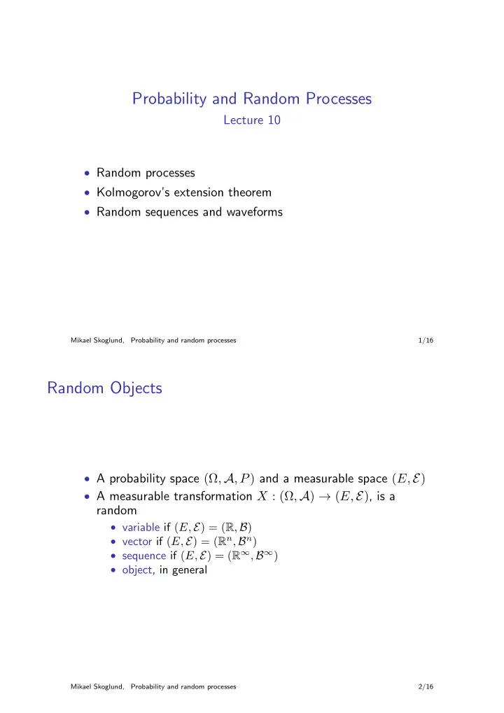
Probability and Random Processes Lecture 10 Random processes - PDF document

Probability and Random Processes Lecture 10 • Random processes • Kolmogorov’s extension theorem • Random sequences and waveforms Mikael Skoglund, Probability and random processes 1/16 Random Objects • A probability space (Ω , A , P ) and a measurable space ( E, E ) • A measurable transformation X : (Ω , A ) → ( E, E ) , is a random • variable if ( E, E ) = ( R , B ) • vector if ( E, E ) = ( R n , B n ) • sequence if ( E, E ) = ( R ∞ , B ∞ ) • object, in general Mikael Skoglund, Probability and random processes 2/16

More on Product Spaces • ( E, E ) a measurable space and T an arbitrary parameter set • E T = { all mappings from T to E } • A measurable rectangle { f ∈ E T : f ( t ) ∈ A t for all t ∈ S } where S is a finite subset S ⊂ T and A t ∈ E for all t ∈ S • For U = { all measurable rectangles } , let E T = σ ( U ) • For t ∈ T , define π t : E T → E to be the evaluation map for any f ∈ E T π t ( f ) = f ( t ) , • Then it holds that E T = σ ( { π t : t ∈ T } ) i.e., E T is the smallest σ -algebra such that all π t : ( E T , E T ) → ( E, E ) , t ∈ T are measurable Mikael Skoglund, Probability and random processes 3/16 • For S ⊂ E define the restriction map π S : E T → E S , via π S ( f ) = f | S • For a finite S ⊂ T and A S ∈ E S , a subset F ⊂ E T is a measurable cylinder if it has the form F = π − 1 S ( A S ) , i.e. F = { f ∈ E T : π S ( f ) ∈ A S , π T \ S ( f ) ∈ E T \ S } = A S × E T \ S • Then it holds that E T = σ ( { all measurable cylinders } ) • A measurable σ -cylinder is a measurable cylinder where the set S ⊂ T is possibly infinite but countable • Then we also have E T = { all measurable σ -cylinders } , • even when T is uncountable, membership f ∈ A ∈ E T imposes restrictions on the values f ( t ) only for countably many t ’s Mikael Skoglund, Probability and random processes 4/16

Random Processes Given (Ω , A , P ) • Random process, definition 1: a collection { X t : t ∈ T } where for each t , X t is a random object X t : (Ω , A ) → ( E, E ) , X − 1 X t : Ω → E, : E → A t for each t , X t maps ω into a value X t ( ω ) ∈ E • Random process, definition 2: a random object X : (Ω , A ) → ( E T , E T ) X − 1 : E T → A X : Ω → E T , X maps each ω into a function X t ( ω ) ∈ E T Mikael Skoglund, Probability and random processes 5/16 Extension Results • Based on definition 2, the process distribution µ X is the distribution of the random object X , that is, A ∈ E T µ X ( A ) = P ( { ω : X t ( ω ) ∈ A } ) , • For a subset S ⊂ T , restricting the process to S means that f ( t ) = X t ( ω ) is restricted to t ∈ S , π S ( f ) = f | S , with corresponding marginal distribution µ X | S on ( E S , E S ) Mikael Skoglund, Probability and random processes 6/16

• Assume that ( E, E , µ t ) are probability spaces for each t ∈ S , where S is a finite subset S ⊂ T , and let ( E S , E S , µ S ) be the corresponding product measure space • Even in the case of an uncountable T , ( E S , E S , µ S ) can be extended to the full space ( E T , E T , µ X ) , in the sense that there exists a unique µ X such that µ X | S ( A ) = µ S ( A ) for all A ∈ E S and any finite S ⊂ T • Proof: The cylinder sets are a semialgebra that generates E T ; a finite product of probability measures is a pre-measure on the cylinders; our previous extension result for product measure can then be extended to a countable S ; finally, the fact that E T is the class of σ -cylinders can be used to extend to the full class E T Mikael Skoglund, Probability and random processes 7/16 • Remember from the definition of product measure, that ( E S , E S , µ S ) corresponds to a process with independent values X t ( ω ) , t ∈ S • Hence we now know how to construct memoryless processes, even for an uncountable T , based on marginal distributions for each finite S • How about completely general µ X ’s? • First result, uniqueness in the general case: for any µ (1) X and X on ( E T , E T ) , if µ (2) µ (1) X | S ( A ) = µ (2) X | S ( A ) for all finite S ⊂ T and A ∈ E S , then µ (1) X = µ (2) X • That is, the finite-dimensional marginal distributions uniquely determine the process distribution, if it exists Mikael Skoglund, Probability and random processes 8/16

Existence: Kolmogorov’s Extension Theorem • A marginal distribution µ X | S , for any finite S ⊂ T , is consistent if µ X | S implies µ X | V for all V ⊂ S • of no concern for product measure, i.e., memoryless marginals. . . (why?) • Extension Theorem: For a given process X from (Ω , A ) to ( E T , E T ) , assume that a consistent distribution µ X | S is specified for any finite subset S ⊂ T . If ( E, E ) is standard, then a unique process distribution µ X exists on ( E T , E T ) that agrees with µ X | S for all finite S ⊂ T • Additional structure is necessary; the result does not hold for all possible ( E, E ) Mikael Skoglund, Probability and random processes 9/16 Discrete-time Real-valued Random Process • Given (Ω , A , P ) , let E = R , E = B , and interpret T as “time” • If T = Z or N , then X is a random sequence or a discrete-time random process, that is { X t } t ∈ T is a countable collection of random variables • ( E, E ) is standard ⇒ Any set of distributions for all random vectors that can be formed by restricting to S = { t 1 , t 2 , . . . , t m } can be extended to a unique process distribution Mikael Skoglund, Probability and random processes 10/16

Continuous-time Real-valued Random Process • Given (Ω , A , P ) , let E = R , E = B , and interpret T as “time” • If T = R or R + , then X is a random waveform or a continuous-time random process, that is { X t } t ∈ T is an uncountable collection of random variables • ( E, E ) is standard, so consistent finite-dimensional marginals can be extended to a unique process distribution on ( E T , E T ) Mikael Skoglund, Probability and random processes 11/16 Finite-energy Waveforms • Introduce the L 2 norm � 1 / 2 �� | g ( t ) | 2 dt � g � = and let L 2 = { Lebesgue measurable f such that � f � 2 < ∞} • Equipped with the inner product � � f, g � = fgdt L 2 is then a separable Hilbert space (with � f � = ( � f, f � ) 1 / 2 ) • With topology T determined by the metric ρ ( f, g ) = � f − g � the space A = ( L 2 , T ) is Polish and ( L 2 , σ ( A )) is standard • The resulting space ( L 2 , σ ( A )) is a model for random finite-energy waveforms Mikael Skoglund, Probability and random processes 12/16

Continuous Waveforms • For a closed interval T ⊂ R , let C ( T ) = { all continuous functions f : T → R } • For g, f ∈ C ( T ) , define the metric ρ ( f, g ) = sup {| f ( t ) − g ( t ) | : t ∈ T } • With topology T determined by ρ , A = ( C ( T ) , T ) is Polish and ( C ( T ) , σ ( A )) is standard • The resulting space ( C ( T ) , σ ( A )) is a model for continuous waveforms on T Mikael Skoglund, Probability and random processes 13/16 Gaussian Processes • Let T = R , R + , Z or N • For any finite S ⊂ T , of size n , let E S = R n and E S the corresponding Borel sets • Define µ X | S on ( E S , E S ) to be the finite Borel measure with density 1 � − 1 � 2( x n − m n ) V − 1 n ( x n − m n ) ′ f n ( x n ) = exp � (2 π ) n | V n | with respect to n -dimensional Lebesgue measure, where V n is a positive-definite n × n matrix and m n ∈ R n Mikael Skoglund, Probability and random processes 14/16

Discrete time • For T = Z or N , the distributions specified by ( m n , V n ) for all finite n uniquely determine a Gaussian sequence { X t } with process distribution µ X • µ X is uniquely specified by knowing m ( t ) = E [ X t ] , V ( k, l ) = E [( X k − m ( k ))( X l − m ( l ))] for all t, k, l ∈ T Mikael Skoglund, Probability and random processes 15/16 Continuous time • For T = R or R + , the distributions specified by ( m n , V n ) for all finite n uniquely determine a Gaussian waveform { X t } with process distribution µ X , specified by m ( t ) = E [ X t ] , V ( s, u ) = E [( X s − m ( s ))( X u − m ( u ))] for all t, s, u ∈ T • Here we need � V ( t, t ) dt < ∞ to get finite-energy waveforms (with probability one) Mikael Skoglund, Probability and random processes 16/16