Probability and Random Processes Lecture 11 Measurable dynamical - PDF document
Probability and Random Processes Lecture 11 Measurable dynamical systems Random processes as dynamical systems Stationarity Ergodic theory Mikael Skoglund, Probability and random processes 1/13 Measurable Dynamical System A
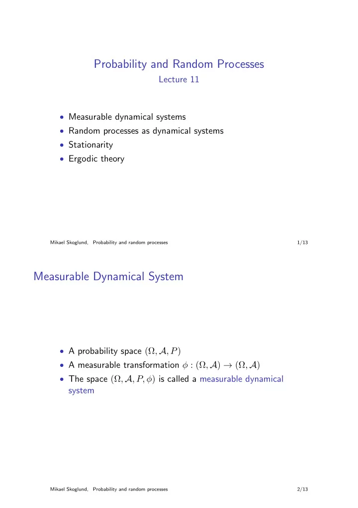
Probability and Random Processes Lecture 11 • Measurable dynamical systems • Random processes as dynamical systems • Stationarity • Ergodic theory Mikael Skoglund, Probability and random processes 1/13 Measurable Dynamical System • A probability space (Ω , A , P ) • A measurable transformation φ : (Ω , A ) → (Ω , A ) • The space (Ω , A , P, φ ) is called a measurable dynamical system Mikael Skoglund, Probability and random processes 2/13
Interpretation • Nature selects an initial state ω = ω 0 • For n ≥ 0 , time acts on ω ∈ Ω to ’move around’ points in Ω , ω n +1 = φ ( ω n ) = { notation } = φω n = φ n +1 ω 0 producing an orbit { ω n } • The orbit is random because ω 0 is selected at random Mikael Skoglund, Probability and random processes 3/13 Random Process as Dynamical System • There are several ways to model a random process as a dynamical system – consider a discrete-time process { X t } , for t ∈ T and with T = N • Approach 1: { X t } is a collection of random variables X t : Ω → R where for each t and ω X t ( ω ) = X ( φ t ω ) for some fixed random variable X • Approach 2: Define φ implicitly on Ω by specifying a time-shift φ ′ on T , i.e., φ ′ ( t ) = t + 1 and φ ′ ( X 0 , X 1 , X 2 , X 3 , . . . ) → ( X 1 , X 2 , X 3 , X 4 , . . . ) Mikael Skoglund, Probability and random processes 4/13
• The model X t ( ω ) = X ( φ t ω ) fits with interpreting { X t } as a collection or random variables • Note that we can also consider ( E T , E T , µ, φ ) , i.e., the evolution of the process is described by φ : E T → E T • for example, φ ( f ( t )) = f ( t + 1) which fits better with the time-shift in approach 2 Mikael Skoglund, Probability and random processes 5/13 Continuous Time • We will focus on systems (Ω , A , P, φ ) interpreting φ as ’one discrete action of time’ – i.e., discrete-time systems • Continuous-time systems can be modeled using a family { φ t } t ∈ Φ of transformations, with Φ = R or R + , such that φ t + s = φ t φ s That is φ t + s ω = φ t φ s ω • The family { φ t } is called a flow • A random waveform can be defined, e.g., as X t ( ω ) = X ( φ t ω ) Mikael Skoglund, Probability and random processes 6/13
Stationarity • A dynamical system (Ω , A , P, φ ) • The system is stationary if P ( A ) = P ( φ − 1 ( A )) , for all A ∈ A (where φ − 1 ( A ) = { ω : φω ∈ A } ⊂ A ) • The system is asymptotically mean stationary (AMS) if the limit n − 1 1 � P ( φ − i ( A )) = ¯ lim P ( A ) n n →∞ i =0 exists pointwise for all A ∈ A • (Ω , A , P, φ ) AMS ⇒ ¯ P is a probability measure and (Ω , A , ¯ P, φ ) is stationary (of course) stationary ⇒ AMS and ¯ P = P Mikael Skoglund, Probability and random processes 7/13 Recurrence • A dynamical system (Ω , A , P, φ ) • A point ω ∈ A is said to be recurrent with respect to A ∈ A if there is a finite N = N A ( ω ) such that φ N ω ∈ A • ω ∈ A ⇒ ω returns to A in finite time • A ∈ A is recurrent if P ( A ) > 0 and P ( { ω ∈ A : ω is not recurrent w.r.t. A } ) = 0 • (Ω , A , P, φ ) is recurrent if all A ∈ A are recurrent • stationary ⇒ recurrent Mikael Skoglund, Probability and random processes 8/13
Ergodicity • A dynamical system (Ω , A , P, φ ) • If A ∈ A is such that φ − 1 ( A ) = A then A is invariant • Let I = { all invariant A ∈ A } • I is a σ -algebra (why?) • (Ω , A , P, φ ) is ergodic if P ( B ) = 1 or 0 for all B ∈ I Mikael Skoglund, Probability and random processes 9/13 The Ergodic Theorem • Theorem: If (Ω , A , P, φ ) is AMS and X is a random variable such that � X ( ω ) d ¯ P < ∞ then n − 1 1 � X ( φ i ω ) = ¯ lim E [ X |I ] n n →∞ i =0 with probability one (under P and ¯ P ), where ¯ E [ X |I ] is conditional expectation w.r.t. ¯ P and where I is the σ -algebra of invariant events Mikael Skoglund, Probability and random processes 10/13
• Let n − 1 1 ¯ � X ( φ n ω ) X = lim n n →∞ i =0 then ¯ X is an I -measurable random variable • Note that � � Xd ¯ ¯ Xd ¯ P = P and that if (Ω , A , P, φ ) , in addition, is ergodic then � ¯ Xd ¯ ¯ X = P -a.e. P, • In particular, if (Ω , A , P, φ ) is stationary and ergodic, then ¯ X = E [ X ] with probability one Mikael Skoglund, Probability and random processes 11/13 Ergodic Decomposition • Fix a standard measurable space (Ω , A ) and φ : Ω → Ω • Assume there is a P such that (Ω , A , P, φ ) is stationary • Then there are a standard space (Γ , S ) , a family { P γ } γ ∈ Γ and a measurable transformation τ : Ω → Γ such that 1 τ is invariant ( τ ( φω ) = τ ( ω )) 2 (Ω , A , P γ , φ ) is stationary and ergodic, for each γ ∈ Γ 3 if τ induces P ∗ ( S ) = P ( τ − 1 ( S )) on (Γ , S ) , then for all A ∈ A � � P ( A ) = P τ ( ω ) ( A ) dP ( ω ) = P γ ( A ) dP ∗ ( γ ) � 4 if f ( ω ) dP ( ω ) < ∞ then � �� � � �� � � fdP = fdP τ ( ω ) dP ( ω ) = fdP γ dP ∗ ( γ ) Mikael Skoglund, Probability and random processes 12/13
• For any stationary (Ω , A , P, φ ) we can decompose P into a mixture of stationary and ergodic components P γ • For A ∈ A , the component in effect is characterized by P γ ( A ) = P ( A | τ = γ ) (regular conditional probability, given the exact outcome γ of the random object τ : (Ω , A ) → (Γ , S ) ) • Interpretation : when time starts, Nature selects which component P γ will be active, with probability P ∗ on (Γ , S ) , ⇒ the output from a stationary system always “looks ergodic,” however we do not know beforehand which ergodic component will be active Mikael Skoglund, Probability and random processes 13/13
Recommend
More recommend
Explore More Topics
Stay informed with curated content and fresh updates.
