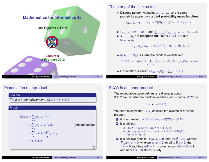
The story of the film so far... Discrete random variables X 1 , . . . - PowerPoint PPT Presentation
The story of the film so far... Discrete random variables X 1 , . . . , X n on the same probability space have a joint probability mass function : Mathematics for Informatics 4a f X 1 ,..., X n ( x 1 , . . . , x n ) = P ( { X 1 = x 1 }
The story of the film so far... Discrete random variables X 1 , . . . , X n on the same probability space have a joint probability mass function : Mathematics for Informatics 4a f X 1 ,..., X n ( x 1 , . . . , x n ) = P ( { X 1 = x 1 } ∩ · · · ∩ { X n = x n } ) Jos´ e Figueroa-O’Farrill f X 1 ,..., X n : R n → [ 0, 1 ] and � x 1 ,..., x n f X 1 ,..., X n ( x 1 , . . . , x n ) = 1 X 1 , . . . , X n are independent if for all 2 � k � n and x i 1 , . . . , x i k , f X i 1 ,..., X ik ( x i 1 , . . . , x i k ) = f X i 1 ( x i 1 ) . . . f X ik ( x i k ) h ( X 1 , . . . , X n ) is a discrete random variable and Lecture 9 � 15 February 2012 E ( h ( X 1 , . . . , X n )) = h ( x 1 , . . . , x n ) f X 1 ,..., X n ( x 1 , . . . , x n ) x 1 ,..., x n Expectation is linear: E ( � i α i X i ) = � i α i E ( X i ) Jos´ e Figueroa-O’Farrill mi4a (Probability) Lecture 9 1 / 23 Jos´ e Figueroa-O’Farrill mi4a (Probability) Lecture 9 2 / 23 Expectation of a product E ( XY ) is an inner product The expectation value defines a real inner product. Lemma If X , Y are two discrete random variables, let us define � X , Y � by If X and Y are independent, E ( XY ) = E ( X ) E ( Y ) . � X , Y � = E ( XY ) Proof. We need to show that � X , Y � satisfies the axioms of an inner product: � E ( XY ) = xyf X , Y ( x , y ) it is symmetric: � X , Y � = E ( XY ) = E ( YX ) = � Y , X � 1 x , y � it is bilinear: 2 = xyf X ( x ) f Y ( y ) (independence) � aX , Y � = E ( aXY ) = a E ( XY ) = a � X , Y � x , y � � � X 1 + X 2 , Y � = E (( X 1 + X 2 ) Y ) = E ( X 1 Y ) + E ( X 2 Y ) = = xf X ( x ) yf Y ( y ) � X 1 , Y � + � X 2 , Y � x y it is positive-definite: if � X , X � = 0, then E ( X 2 ) = 0, whence 3 = E ( X ) E ( Y ) � x x 2 f ( x ) = 0, whence xf ( x ) = 0 for all x . If x � = 0, then f ( x ) = 0 and thus f ( 0 ) = 1. In other words, P ( X = 0 ) = 1 and hence X = 0 almost surely. Jos´ e Figueroa-O’Farrill mi4a (Probability) Lecture 9 3 / 23 Jos´ e Figueroa-O’Farrill mi4a (Probability) Lecture 9 4 / 23
Additivity of variance for independent variables Covariance How about the variance Var ( X + Y ) ? Definition The covariance of two discrete random variables is Var ( X + Y ) = E (( X + Y ) 2 ) − E ( X + Y ) 2 Cov ( X , Y ) = E ( XY ) − E ( X ) E ( Y ) = E ( X 2 + 2 XY + Y 2 ) − ( E ( X ) + E ( Y )) 2 = E ( X 2 ) + 2 E ( XY ) + E ( Y 2 ) − E ( X ) 2 − 2 E ( X ) E ( Y ) − E ( Y ) 2 = Var ( X ) + Var ( Y ) + 2 ( E ( XY ) − E ( X ) E ( Y )) Letting µ X and µ Y denote the means of X and Y , respectively, Cov ( X , Y ) = E (( X − µ X )( Y − µ Y )) Theorem Indeed, If X and Y are independent discrete random variables E (( X − µ X )( Y − µ Y )) = E ( XY ) − E ( µ X Y ) − E ( µ Y X ) + E ( µ X µ Y ) Var ( X + Y ) = Var ( X ) + Var ( Y ) = E ( XY ) − µ X µ Y Jos´ e Figueroa-O’Farrill mi4a (Probability) Lecture 9 5 / 23 Jos´ e Figueroa-O’Farrill mi4a (Probability) Lecture 9 6 / 23 Example (Max and min for two fair dice) Definition Two discrete random variables X and Y are said to be We roll two fair dice. Let X and Y denote their scores. uncorrelated if Cov ( X , Y ) = 0. Independence says that Cov ( X , Y ) = 0. Consider however the new variables U = min ( X , Y ) and V = max ( X , Y ) : U 1 2 3 4 5 6 V 1 2 3 4 5 6 Warning 1 1 1 1 1 1 1 1 1 2 3 4 5 6 Uncorrelated random variables need not be independent! 2 1 2 2 2 2 2 2 2 2 3 4 5 6 3 1 2 3 3 3 3 3 3 3 3 4 5 6 Counterexample 4 1 2 3 4 4 4 4 4 4 4 4 5 6 Suppose that X is a discrete random variable with probability 5 1 2 3 4 5 5 5 5 5 5 5 5 6 mass function symmetric about 0; that is, f X (− x ) = f X ( x ) . Let 6 1 2 3 4 5 6 6 6 6 6 6 6 6 Y = X 2 . Clearly X , Y are not independent: f ( x , y ) = 0 unless y = x 2 even if f X ( x ) f Y ( y ) � = 0. However they are uncorrelated: E ( U ) = 91 36 , E ( U 2 ) = 301 36 , E ( V ) = 161 36 , E ( V 2 ) = 791 36 , E ( UV ) = 49 4 � � 2 E ( XY ) = E ( X 3 ) = x 3 f X ( x ) = 0 � ⇒ Var ( U ) = Var ( V ) = 2555 35 and Cov ( U , V ) = = 1296 36 x and similarly E ( X ) = 0, whence E ( X ) E ( Y ) = 0. Jos´ e Figueroa-O’Farrill mi4a (Probability) Lecture 9 7 / 23 Jos´ e Figueroa-O’Farrill mi4a (Probability) Lecture 9 8 / 23
An alternative criterion for independence The Cauchy–Schwarz inequality The above counterexample says that the following implication Recall that � X , Y � = E ( XY ) is an inner product. cannot be reversed: Cauchy–Schwarz inequality : Every inner product obeys the X , Y independent = ⇒ E ( XY ) = E ( X ) E ( Y ) � X , Y � 2 � � X , X � � Y , Y � which in terms of expectations is However, one has the following E ( XY ) 2 � E ( X 2 ) E ( Y 2 ) Theorem Two discrete random variables X and Y are independent if and Now, only if Cov ( X , Y ) 2 = E (( X − µ X )( Y − µ Y )) 2 � E (( X − µ X ) 2 ) E (( Y − µ Y ) 2 ) E ( g ( X ) h ( Y )) = E ( g ( X )) E ( h ( Y )) for all functions g , h . whence Cov ( X , Y ) 2 � Var ( X ) Var ( Y ) The proof is not hard, but we will skip it. Jos´ e Figueroa-O’Farrill mi4a (Probability) Lecture 9 9 / 23 Jos´ e Figueroa-O’Farrill mi4a (Probability) Lecture 9 10 / 23 Correlation Example (Max and min for two fair dice – continued) previous example , we now simply compute Let X and Y be two discrete random variables with means µ X Continuing with the and µ Y and standard deviations σ X , σ Y . The correlation ρ ( X , Y ) � = 35 2 of X and Y is defined by Cov ( U , V ) 2555 = 35 ρ ( U , V ) = 73 . � 36 2 36 2 Var ( U ) Var ( V ) ρ ( X , Y ) = Cov ( X , Y ) σ X σ Y From the Cauchy–Schwarz inequality, we see that Remark The funny normalisation of ρ ( X , Y ) is justified by the following: ρ ( X , Y ) 2 � 1 = ⇒ − 1 � ρ ( X , Y ) � 1 ρ ( αX + β , γY + δ ) = sign ( αγ ) ρ ( X , Y ) Hence the correlation is a number between − 1 and 1: a correlation of 1 suggests a linear relation with positive which follows from slope between X and Y , Cov ( αX + β , γY + δ ) = αγ Cov ( X , Y ) whereas a correlation of − 1 suggests a linear relation with negative slope. and σ αX + β = | α | σ X and σ γY + δ = | γ | σ Y . Jos´ e Figueroa-O’Farrill mi4a (Probability) Lecture 9 11 / 23 Jos´ e Figueroa-O’Farrill mi4a (Probability) Lecture 9 12 / 23
Markov’s inequality Example Theorem (Markov’s inequality) A factory produces an average of n items every week. What can be said about the probability that this week’s production Let X be a discrete random variable shall be at least 2 n items? taking non-negative values. Then Let X be the discrete random variable counting the number of P ( X � a ) � E ( X ) items produced. Then by Markov’s inequality a P ( X � 2 n ) � n 2 n = 1 2 . So I wouldn’t bet on it! Proof. Markov’s inequality is not terribly sharp; e.g., � � � E ( X ) = x P ( X = x ) = x P ( X = x ) + x P ( X = x ) P ( X � E ( X )) � 1 . x � 0 0 � x<a x � a � � x P ( X = x ) � a P ( X = x ) = a P ( X � a ) � x � a x � a It has one interesting corollary, though. Jos´ e Figueroa-O’Farrill mi4a (Probability) Lecture 9 13 / 23 Jos´ e Figueroa-O’Farrill mi4a (Probability) Lecture 9 14 / 23 Chebyshev’s inequality Example Back to the factory in the previous example, let the average be Theorem n = 500 and the variance in a week’s production is 100, then Let X be a discrete random variable with what can be said about the probability that this week’s mean µ and variance σ 2 . Then for any production falls between 400 and 600? ε > 0 , By Chebyshev’s, P ( | X − µ | � ε ) � σ 2 ε 2 σ 2 1 P ( | X − 500 | � 100 ) � 100 2 = 100 whence Proof. Notice that for ε > 0, | X − µ | � ε if and only if ( X − µ ) 2 � ε 2 , so P ( | X − 500 | < 100 ) = 1 − P ( | X − 500 | � 100 ) P ( | X − µ | � ε ) = P (( X − µ ) 2 � ε 2 ) 100 = 99 1 � 1 − 100 . � E (( X − µ ) 2 ) = σ 2 So pretty likely! (by Markov’s) ε 2 ε 2 Jos´ e Figueroa-O’Farrill mi4a (Probability) Lecture 9 15 / 23 Jos´ e Figueroa-O’Farrill mi4a (Probability) Lecture 9 16 / 23
Recommend
More recommend
Explore More Topics
Stay informed with curated content and fresh updates.


