Lecture 6 : Discrete Random Variables and Probability Distributions - PDF document

Lecture 6 : Discrete Random Variables and Probability Distributions 0/ 32

Go to “BACKGROUND COURSE NOTES” at the end of my web page and download the file distributions . Today we say goodbye to the elementary theory of probability and start Chapter 3 . We will open the door to the application of algebra to probability theory by introduction the concept of “random variable”. 1/ 32 Lecture 6 : Discrete Random Variables and Probability Distributions

What you will need to get from it (at a minimum) is the ability to do the following “Good Citizen Problems ”. I will give you a probability mass function P ( X ) . You will be asked to compute (i) The expected value (or mean ) E ( X ) . (ii) The variance V ( X ) . (iii) The cumulative distribution function F ( x ) . You will learn what these words mean shortly. 2/ 32 Lecture 6 : Discrete Random Variables and Probability Distributions

Mathematical Definition Let S be the sample space of some experiment (mathematically a set S with a probability measure P ). A random variable X is a real-valued function on S . Intuitive Idea A random variable is a function, whose values have probabilities attached. Remark To go from the mathematical definition to the “intuitive idea” is tricky and not really that important at this stage. 3/ 32 Lecture 6 : Discrete Random Variables and Probability Distributions

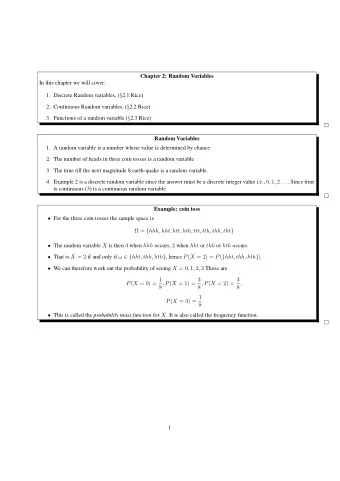
The Basic Example Flip a fair coin three times so S = { HHH , HHT , HTH , HTT , THH , THT , TTH , TTT } Let X be function on X given by X = number of heads so X is the function given by { HHH , HHT , HTH , HTT , THH , THT , TTH , TTT } ↓ ↓ ↓ ↓ ↓ ↓ ↓ ↓ 3 2 2 1 2 1 1 0 What are P ( X = 0 ) , P ( X = 3 ) , P ( X = 1 ) , P ( X = 2 ) 4/ 32 Lecture 6 : Discrete Random Variables and Probability Distributions

Answers Note ♯ ( S ) = 8 P ( X = 0 ) = P ( TTT ) = 1 8 P ( X = 1 ) = P ( HTT ) + P ( THT ) + P ( TTH ) = 3 8 P ( X = 2 ) = P ( HHT ) + P ( HTH ) + P ( THH ) = 3 8 P ( X = 3 ) = P ( HHH ) = 1 8 We will tabulate this Value X 0 1 2 3 1 3 3 1 Probability of the value P ( X = x ) 8 8 8 8 Get used to such tabular presentations. 5/ 32 Lecture 6 : Discrete Random Variables and Probability Distributions

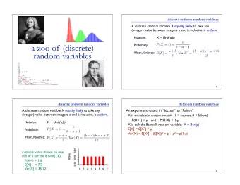
Rolling a Die Roll a fair die, let X = the number that comes up So X takes values 1 , 2 , 3 , 4 , 5 , 6 each with probability 1 6. X 1 2 3 4 5 6 1 1 1 1 1 1 P ( X = x ) 6 6 6 6 6 6 This is a special case of the discrete uniform distribution where X takes values 1 , 2 , 3 , . . . , n each with probability 1 n (so roll a fair die with n faces”). 6/ 32 Lecture 6 : Discrete Random Variables and Probability Distributions

Bernoulli Random Variable Usually random variables are introduced to make things numerical. We illustrate this by an important example - page 8. First meet some random variables. Definition (The simplest random variable(s)) The actual simplest random variable is a random variable in the technical sense but isn’t really random. It takes one value (let’s suppose it is 0 ) with probability one X 0 P ( X = 0 ) 1 Nobody ever mentions this because it is too simple - it is deterministic. 7/ 32 Lecture 6 : Discrete Random Variables and Probability Distributions

The simplest random variable that actually is random takes TWO values, let’s suppose they are 1 and 0 with probabilities p and q . Since X has to be either 1 on 0 we must have p + q = 1 . So we get X 0 1 P ( X = x ) q p This called the Bernoulli random variable with parameter p . So a Bernoulli random variable is a random variable that takes only two values 0 and 1. 8/ 32 Lecture 6 : Discrete Random Variables and Probability Distributions

Where do Bernoulli random variables come from? We go back to elementary probability. Definition A Bernoulli experiment is an experiment which has two outcomes which we call (by convention) “success” S and failure F. Example Flipping a coin. We will call a head a success and a tail a failure. Z Often we call a “success” something that is in fact for from an actual success- e.g., a machine breaking down. 9/ 32 Lecture 6 : Discrete Random Variables and Probability Distributions

In order to obtain a Bernoulli random variable if we first assign probabilities to S and F by P ( S ) = p and P ( F ) = q so again p + q = 1. Thus the sample space of a a Bernoulli experiment will be denoted S (note that that the previous caligraphic S is different from Roman S) and is given by S = { S , F } . We then obtain a Bernoulli random variable X on S by defining X ( S ) = 1 and X ( F ) = 0 so P ( X = 1 ) = P ( S ) = p and P ( X = 0 ) = P ( F ) = q . 10/ 32 Lecture 6 : Discrete Random Variables and Probability Distributions

Discrete Random Variables Definition A subset S of the red line R is said to be discrete if for every whole number n there are only finitely many elements of S in the interval [ − n , n ] . 0 So a finite subset of R is discrete but so is the set of integers Z . 11/ 32 Lecture 6 : Discrete Random Variables and Probability Distributions

Remark The definition in the text on page 98 is wrong. The set of rational numbers Q is countably infinite but is not discrete. This is not important for this course but I find it almost unbelievablel that the editors of this text would allow such an error to run through nine editions of the text. Definition A random variable is said to be discrete if its set of possible values is a discrete set. A possible value means a value x 0 so that P ( X = x 0 ) � 0. 12/ 32 Lecture 6 : Discrete Random Variables and Probability Distributions

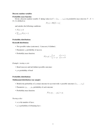
Definition The probability mass function (abbreviated pmf) of a discrete random variable X is the function p X defined by p X ( x ) = P ( X = x ) We will often write p ( x ) instead of P X ( x ) . Note (i) p ( x ) ≥ 0 � p ( x ) = 1 (ii) all possible X (iii) p ( x ) = 0 for all X outside a discrete set. 13/ 32 Lecture 6 : Discrete Random Variables and Probability Distributions

Graphical Representations of Proof’s There are two kinds of graphical representations of proof’s, the “line graph” and the “probability histogram”. We will illustrate them with the Bernoulli distribution with parameter P . X 1 0 P ( X = x ) p q table line graph 1 0 histogram 0 1 14/ 32 Lecture 6 : Discrete Random Variables and Probability Distributions

We also illustrate these for the basic example (pg. 5). X 0 1 2 3 1 3 3 1 P ( X = x ) table 8 8 8 8 0 1 2 3 0 1 2 3 15/ 32 Lecture 6 : Discrete Random Variables and Probability Distributions

The Cumulative Distribution Function The cumulative distribution function F X (abbreviated cdf) of a discrete random variable X is defined by F X ( x ) = P ( X ≤ x ) We will often write F ( x ) instead of F X ( x ) . Bank account analogy Suppose you deposit 1000 at the beginning of every month. 1000 ``live graph'' 16/ 32 Lecture 6 : Discrete Random Variables and Probability Distributions

The “line graph” of your deposits is on the previous page. We will use t (time as our variable). Let F ( t ) = the amount you have accumulated at time t . What does the graph of F look like? 5000 etc 17/ 32 Lecture 6 : Discrete Random Variables and Probability Distributions

It is critical to observe that whereas the deposit function on page 15 is zero for all real numbers except 12 numbers (Here I am replacing the symbols for the months e.g. J by the numbers 1 through 12) the cumulative distribution function is never zero between 1 and ∞ . You would be very upset if you walked into the bank on July 5 th and they told you your balance was zero - you never took any money out. Once your balance was nonzero it was never zero thereafter. 18/ 32 Lecture 6 : Discrete Random Variables and Probability Distributions

Back to Probability The cumulative distribution F ( x ) is “the total probability you have accumulated when you get to x ”. Once it is nonzero it is never zero again ( p ( x ) ≥ 0 means “you never take any probability out”). To write out p ( x ) in formulas you will need several (many) formulas. There should never be EQUALITIES in you formulas only INEQUALITIES. 19/ 32 Lecture 6 : Discrete Random Variables and Probability Distributions

The cdf for the Basic Example We have line graph of 0 2 3 1 So we start accumulation probability at X = 0 Ordinary Graph of F 1 3 0 1 2 20/ 32 Lecture 6 : Discrete Random Variables and Probability Distributions

Formulas for F   0 x ≤ 0       1   0 ≤ x < 1     8         4 1 ≤ x < 2     ←− be careful 8     7   1 ≤ x < 3       8         1 3 ≤ x     You can see you here to be careful about the inequalities on the right-hand side. 21/ 32 Lecture 6 : Discrete Random Variables and Probability Distributions

The relation between p and F We will need the relation between the probability mass function p ( x ) and the cumulative distribution function F ( x ) . Recall that if F ( x ) is a function of an integer variable x then the backward difference function (discrete derivative) ∆ F of F is defined by ∆ F ( x ) = F ( x ) − F ( x − 1 ) . The relation we want is Theorem 1 p ( x ) = ∆ F ( x ) 22/ 32 Lecture 6 : Discrete Random Variables and Probability Distributions