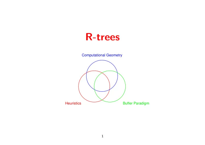
R-trees Computational Geometry Heuristics Buffer Paradigm 1 - PowerPoint PPT Presentation
R-trees Computational Geometry Heuristics Buffer Paradigm 1 Spatial Data Spatial data: points, lines, polygons/polyhedra in R d . For simplicity: assume d = 2 . Typical queries: Point: All objects containing query point Intersection: All
R-trees Computational Geometry Heuristics Buffer Paradigm 1
Spatial Data Spatial data: points, lines, polygons/polyhedra in R d . For simplicity: assume d = 2 . Typical queries: Point: All objects containing query point Intersection: All objects intersecting query object Enclosure: All objects containing query object Spatial Join: All intersections between stored objects and query set of objects Example: windowing in GIS. 2
R-trees Approximate objects by Bounding Box: [Guttman, 84] R-tree = B-tree where • Leaves store objects and their BBs. • Internal nodes store for each child a BB containing all objects in that subtree. 3
Searching in R-trees Example: Point Query Search recursively in all subtrees of node where BB contains the query point. Observe: • Worst case query time: Θ( N ) ! • Average case performance depends heavily on distribution of objects in leaves. Heuristic data structure. 4
Static R-Trees Build (“bulk load” in database community): 1. Distribute objects in leaves ( ⇔ assign linear order). 2. Build R-tree bottom up. Number of I/O’s: 1. O (Sort( N )) 2. O (Scan( N )) Query efficiency: depends heavily on the linear order. Example: random distribution in leaves ⇒ most leaves has BB close to BB of entire set of objects ⇒ queries inefficient. Goal: linear order where objects close in order ⇔ close in Euclidean distance. 5
Space Filling Curves The z -curve: Comparing ( x, y ) and ( x ′ , y ′ ) having binary expansions ( x 1 x 2 . . . x k , y 1 y 2 . . . y k ) and ( x ′ 1 x ′ 2 . . . x ′ k , y ′ 1 y ′ 2 . . . y ′ k ) : Compare y 1 and y ′ 1 , then x 1 and x ′ 1 , then y 2 and y ′ 2 . . . � Compare y 1 x 1 y 2 x 2 . . . x k and y ′ 1 x ′ 1 y ′ 2 x ′ 2 . . . x ′ k “Bit interleaving” 6
Space Filling Curves The Hilbert-curve: Note: subpattern = pattern flipped along a diagonal. Generates four possibilities (as flip 2 1 = flip 2 2 = ID and as flip 1 flip 2 = flip 2 flip 1 ). Comparing ( x, y ) and ( x ′ , y ′ ) having binary expansions ( x 1 x 2 . . . x k , y 1 y 2 . . . y k ) and ( x ′ 1 x ′ 2 . . . x ′ k , y ′ 1 y ′ 2 . . . y ′ k ) : Top level: Compare x 1 and x ′ 1 , then y 1 and y ′ 1 . Advance to next bit, choosing proper variant of this scheme. 7
Space Filling Curves and R-Trees Choose ordering in leaves by sorting midpoints of bounding boxes of objects according to position on some space filling curve. Empirically: A static R-tree build this way has good query time in practice. 8
Dynamic R-trees Insert: We need two subroutines: Route() Given a node v and a new object x , decide which subtree of v that x should belong to. Split() Given a node v that is overflowing, decide how to split the subtrees in two groups. Various heuristics for these have been proposed, based on minimizing various properties of changed BBs (total area, area not used by objects, circumference, overlap with siblings BB, . . . ). Bottom line: ∃ fast heuristics giving good query times in practice. 9
Buffered R-Trees [AHVV, 99] Add buffers of size Θ( M ) to layers i · log B ( m/ 4) , for i = 1 , 2 , . . . . log B ( m/ 4) Principle and analysis: exactly as for buffer trees (using Route and Split ) Advantage: Efficient bulk updates and queries. For Θ( N ) size bulks: Number of I/O’s is O ( 1 B log m ( N )) per insert instead of Θ(log B ( N )) . 10
Buffered R-Trees Similar statements for queries and deletions (see paper). Note that spatial join is a bulk query. Empirically: Faster bulk insertions than for previous proposals. Query time in resulting structure competitive with repeated insertions. 11
Recommend
More recommend
Explore More Topics
Stay informed with curated content and fresh updates.
