Program Construction, continued Roland Backhouse March 19, 2001 2 - PowerPoint PPT Presentation

1 Program Construction, continued Roland Backhouse March 19, 2001

2 Outline • Conditional Statements • Sequential Composition

3 Sequential Composition Suppose a programming problem is specified by giving a precondition P and postcondition Q . We are required to construct a program statement S to satisfy { P } S { Q } . We can decompose this problem by inventing a suitable intermediate condition R and then constructing program statements S1 and S2 such that { P } S1 { R } and { R } S2 { Q } .

4 Rule of Sequential Composition { P } S1 ; S2 { Q } { P } S1 { R } ∧ { R } S2 { Q } . ⇐ Methodology 1. Invent a suitable intermediate condition R . 2. Invent statement S1 . 3. Invent statement S2 .

5 The skip statement Sequential composition is associative. That is, it does not matter whether we read S ; T ; U as ( S ; T ) ; U or as S ;( T ; U ) . Sequential composition also has a unit. It is the “do-nothing” statement. We denote it by skip . skip ; S = S = S ; skip

6 The skip rule { P } skip { Q } ≡ P ⇒ Q . Weakening In most cases, skip is not explicit (think of it as being written with zero amount of ink). The skip rule is thus most often used in the form: { P } { Q } ≡ P ⇒ Q . So, if two bracketed assertions appear consecutively in a program the meaning is that the first assertion is always true at that point in the program’s execution but may be weakened to the second assertion.

7 Weakest Preconditions The assignment rule gives the weakest precondition that will guarantee a given postcondition after execution of an assignment. Example { 0 <k } { 0 <k + 1 } k := k + 1 { 0 <k } . The condition 0 <k + 1 is the weakest condition guaranteeing that 0 <k after the assignment k := k + 1 . The condition 0 <k is stronger than the condition 0 <k + 1 . So, using the rule of sequential composition, with S1 the skip statement, combined with the weakening rule, we infer that { 0 <k } k := k + 1 { 0 <k } .

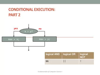
8 Conditional Statements The most common form of conditional statement is the if-then-else statement. A statement of the form if b then S else T is executed by evaluating the boolean expression b ; then if b evaluates to true the statement S is executed, otherwise (“else”) the statement T is executed. For example, the statement if x ≤ 0 then y := − x else y := x assigns to y the absolute value of x .

9 An Asymmetry The use of “ else ” leads to an asymmetry in the branches of a conditional statement. In the evaluation of the absolute value of x , the case x = 0 can be handled by either the assignment y := − x or by the asssignment y := x ; it doesn’t matter which is chosen. The asymmetry becomes more pronounced when there are more cases to be considered, as in for example if a [ i ] <b [ j ] then i := i + 1 else if b [ j ] <a [ i ] then j := j + 1 else i,j := i + 1 ,j + 1 .

10 Guarded Commands A modest improvement can be obtained if each branch of a conditional statement is “guarded” with the condition under which it is executed. An example is the statement if x ≤ 0 → y := − x ✷ x ≥ 0 → y := x fi . The conditional statement is executed by evaluating both the guards and then executing any one of the statements whose guard evaluates to true . Note that this makes evaluation of a conditional statement nondeterministic in that it may be the case that both guards evaluate to true . This nondeterminism is an advantage of the guarded command style of writing conditionals. It saves the programmer from making arbitrary and possibly confusing distinctions.

11 Example if a [ i ] <b [ j ] → i := i + 1 ✷ a [ i ] = b [ j ] → i,j := i + 1 ,j + 1 ✷ a [ i ] >b [ j ] → j := j + 1 fi . If-then Statement if b → S ✷ ¬ b → skip fi .

12 Reasoning about conditionals Consider { P } if b1 → S1 ✷ b2 → S2 fi { Q } . Execution of statement S1 is begin in a state satisfying P ∧ b1 and statement S2 in a state satisfying P ∧ b2 . Thus: { P } if b1 → { P ∧ b1 } S1 { Q } ✷ b2 → { P ∧ b2 } S2 { Q } fi { Q } .

13 Example { true } if x ≤ 0 → { true ∧ x ≤ 0 } y := − x { y = | x | } ✷ x ≥ 0 → { true ∧ x ≥ 0 } y := x { y = | x | } fi { y = | x | } . Since it is the case that either x ≤ 0 or x ≥ 0 , at least one of the two assignments will be chosen for execution. The correctness of the conditional statement is thus reduced to { x ≤ 0 } y := − x { y = | x | } and { x ≥ 0 } y := x { y = | x | } .

14 Using the assignment axiom, we have { − x = | x | } y := − x { y = | x | } . But, it is indeed a property of absolute values that x ≤ 0 ≡ − x = | x | . Substituting equals for equals ( x ≤ 0 for − x = | x | ) we have thus verified the correctness of the first assignment. Also, again using the assignment axiom, { x = | x | } y := x { y = | x | } . But x ≥ 0 ≡ x = | x | . Substituting equals for equals again (this time x ≥ 0 for x = | x | ) the second assignment is valid. We conclude that the conditional statement correctly assigns the absolute value of x to y .

15 The Conditional Rule { P } if b1 → S1 ✷ b2 → S2 fi { Q } is equivalent to the conjunction of three propositions: P ⇒ b1 ∨ b2 , { P ∧ b1 } S1 { Q } , and { P ∧ b2 } S2 { Q } .

16 Constructing conditional statements Suppose a specification of a program statement S is given in terms of a precondition P and a postcondition Q . Then we can meet the specification in three steps: (a) Split the precondition into two (or possibly more) conditions b1 and b2 . Formally, “splitting the precondition” means identifying b1 and b2 such that P ⇒ b1 ∨ b2 . (b) Construct a program statement S1 that guarantees termination in a state satisfying Q given the precondition P ∧ b1 . (c) Construct a program statement S2 that guarantees termination in a state satisfying Q given the precondition P ∧ b2 .

17 Computing the Maximum Problem : Assign the maximum of x and y to z (all assumed to be real values). Precondition : true . Postcondition : z = x ↑ y . Maximum has the following elementary properties: x ↑ y = x ≡ y ≤ x , (1) and x ↑ y = y ≡ x ≤ y . (2) Since also x ≤ y ∨ y ≤ x we are led to consider splitting the problem into two cases, the case that x ≤ y and the case that y ≤ x .

18 So our goal is to calculate expressions e1 and e2 such that { true } if x ≤ y → z := e1 ✷ y ≤ x → z := e2 fi { z = x ↑ y } . That is, e1 and e2 must satisfy { x ≤ y } z := e1 { z = x ↑ y } and { y ≤ x } z := e2 { z = x ↑ y } .

19 Using the assignment axiom we calculate that { e = x ↑ y } z := e { z = x ↑ y } . In particular, { x = x ↑ y } z := x { z = x ↑ y } . Thus by (1), { y ≤ x } z := x { z = x ↑ y } . Similarly, using the assignment axiom and (2), { x ≤ y } z := y { z = x ↑ y } . We have thus determined expressions e1 and e2 and conclude that: { true } if x ≤ y → z := y ✷ y ≤ x → z := x fi { z = x ↑ y } .

20 Combining the Rules An Example Suppose that a programming language does not have a direct implementation of integer division by 2 . However, it is required to write a program that will implement the assignment m := m ÷ 2 for a given positive integer m . Formally, using ghost variable M to record the initial value of m , the problem is to construct a statement S such that { 0 ≤ m = M } S { m = M ÷ 2 } .

21 Permitted Operations Let us suppose that the language does have a division-by-two operation in the case that the supplied argument is positive and even. Let us denote this operation by rot (short for rotate ). Then, what we may assume is that the function rot satisfies, for all k , 0 ≤ k ∧ even .k ⇒ rot .k = k ÷ 2 . (3) That is rot .k correctly computes the integer division k ÷ 2 in the case that k is positive and even. We also assume that the language implements a test even that determines whether a given argument k is even or not. Finally, we assume that the language has an operation dec (short for decrement ) that subtracts one from a given strictly positive integer. That is, dec satisfies, for all k , (4) 0 <k ⇒ dec .k = k − 1 .

22 Applying Sequential Composition At some stage the program must compute rot .k for some k . This operation computes k ÷ 2 reliably only when k is even. (See (4).) The input value M is not necessarily even so it’s reasonable to seek a program that ensures that m gets an even value and then assigns rot .m to m . That is, we use the rule of sequential composition to replace the original problem by the problem of determining a statement S and an intermediate condition P satisfying { 0 ≤ m = M } S { 0 ≤ m ∧ even .m ∧ P } . (5) and { 0 ≤ m ∧ even .m ∧ P } m := rot .m { m = M ÷ 2 } . (6)

23 Calculating the Intermediate Condition Applying the assignment axiom, we have: { rot .m = M ÷ 2 } m := rot .m { m = M ÷ 2 } . So P must satisfy: 0 ≤ m ∧ even .m ∧ P ⇒ rot .m = M ÷ 2 . Recalling the given property of rot : 0 ≤ m ∧ even .m ⇒ rot .m = m ÷ 2 . it is clear that m ÷ 2 = M ÷ 2 P ≡ will do.

24 Specification of S Substituting the calculated value for P in (7) and (6) gives us { 0 ≤ m ∧ even .m ∧ m ÷ 2 = M ÷ 2 } m := rot .m { m = M ÷ 2 } and the specification of S : { 0 ≤ m = M } S { 0 ≤ m ∧ even .m ∧ m ÷ 2 = M ÷ 2 } . In words, S must compute a positive, even number m which has the same integer division by two as M .