PROFILE OF RANDOM TREES Michael Drmota Institute of Discrete - PowerPoint PPT Presentation
PROFILE OF RANDOM TREES Michael Drmota Institute of Discrete Mathematics and Geometry Vienna University of Technology A 1040 Wien, Austria michael.drmota@tuwien.ac.at http://www.dmg.tuwien.ac.at/drmota/ LIPN Paris Nord, February 24, 2015
PROFILE OF RANDOM TREES Michael Drmota Institute of Discrete Mathematics and Geometry Vienna University of Technology A 1040 Wien, Austria michael.drmota@tuwien.ac.at http://www.dmg.tuwien.ac.at/drmota/ LIPN Paris Nord, February 24, 2015
Contents 0. Profile of Trees I. Galton-Watson Trees II. Search Trees III. Digital Trees
Book Michael Drmota, Random Trees , Springer, Wien-New York, 2009.
Profile of Trees Rooted tree root
Profile of Trees Rooted tree root
Profile of Trees I T ( k ) ... number of nodes at distance k from the root ( I T ( k )) k ≥ 0 ... profile of T ( I T ( s ) , s ≥ 0) ... linearly interpolated profile of T ( I n,k ) k ≥ 0 ... profile in a random tree of size n k L(k)
Profile of Trees Parameters of interest: • Profile I n,k (number of nodes at depth k ) • Depth of a random node: D n • Internal path length : L n (sum of all distances to the root) • Height H n
Profile of Trees Relations to the profile I n,k : • Pr { D n = k } = 1 n E I n,k � • L n = kI n,k k ≥ 0 • H n = max { k ≥ 0 : I n,k > 0 } • The profile describes the shape of the tree.
Contents 0. Profile of Trees I. Galton-Watson Trees II. Search Trees III. Digital Trees
Galton-Watson Trees Catalan trees root rooted, ordered (or plane) tree
Galton-Watson Trees g n x n � Catalan trees. g n = number of Catalan trees of size n ; G ( x ) = n ≥ 1 ... = + + + + x G ( x ) = x (1 + G ( x ) + G ( x ) 2 + · · · ) = 1 − G ( x ) G ( x ) = 1 − √ 1 − 4 x 4 n − 1 g n = 1 � 2 n − 2 � ∼ = √ π · n 3 / 2 ⇒ 2 n n − 1 (Catalan numbers)
Galton-Watson Trees Catalan trees with singularity analysis G ( x ) = 1 − √ 1 − 4 x √ = 1 2 − 1 1 − 4 x 2 2 2 · 4 n n − 3 / 2 4 n − 1 g n ∼ − 1 = = √ π · n 3 / 2 ⇒ Γ( − 1 2 )
Galton-Watson Trees Galton-Watson branching process ξ ... offspring distribution, ϕ k = P { ξ = k } , ϕ 0 > 0
Galton-Watson Trees Galton-Watson branching process ξ ... offspring distribution, ϕ k = P { ξ = k } , ϕ 0 > 0
Galton-Watson Trees Galton-Watson branching process ξ ... offspring distribution, ϕ k = P { ξ = k } , ϕ 0 > 0
Galton-Watson Trees Galton-Watson branching process ξ ... offspring distribution, ϕ k = P { ξ = k } , ϕ 0 > 0
Galton-Watson Trees Galton-Watson branching process ξ ... offspring distribution, ϕ k = P { ξ = k } , ϕ 0 > 0
Galton-Watson Trees Galton-Watson branching process ξ ... offspring distribution, ϕ k = P { ξ = k } , ϕ 0 > 0
Galton-Watson Trees Galton-Watson branching process . ( Z k ) k ≥ 0 Z 0 = 1, and for k ≥ 1 Z k − 1 ξ ( k ) � Z k = , j j =1 where the ( ξ ( k ) ) k,j are iid random variables distributed as ξ . j Z k ... number of nodes in k -th generation Z = Z 0 + Z 1 + Z 2 + · · · ... total progeny
Galton-Watson Trees Generating functions y n x n � y n = P { Z = n } , y ( x ) = n ≥ 1 Φ( w ) = E w ξ = ϕ k w k � k ≥ 0 y ( x ) = x Φ( y ( x )) = ⇒ Conditioned Galton-Watson tree GW-branching process conditioned on the total progeny Z = n .
Galton-Watson Trees Example . P { ξ = k } = 2 − k − 1 , Φ( w ) = 1 / (2 − w ) = all trees of size n have the same probability ⇒ = conditioned GW-tree of size n is the same model as the Catalan ⇒ tree model (with the uniform distribution on trees of size n ) Example . Φ( w ) = 1 2 (1 + w ) 2 : binary trees with n internal nodes. Example . Φ( w ) = 1 3 (1 + w + w 2 ): Motzkin trees Example . Φ( w ) = e w − 1 : Cayley trees
Galton-Watson Trees Depth-First-Search – Rooted trees and discrete excursions x(i) i Bijection between Catalan trees Dyck paths ← → random trees of size n random Dyck paths of length 2 n ← →
Galton-Watson Trees Depth-First-Search Brownian excursion ( e ( t ) , 0 ≤ t ≤ 1) 1.6 1.4 1.2 1 0.8 0.6 0.4 0.2 0 -0.2 0 0.2 0.4 0.6 0.8 1 Rescaled Brownian motion between 2 zeros. Random function in C [0 , 1].
Depth-First-Search Kaigh’s Theorem ( X n ( t ) , 0 ≤ t ≤ 2 n ) ... random Dyck path of length 2 n . � � 1 d √ 2 nX n (2 nt ) , 0 ≤ t ≤ 1 → ( e ( t ) , 0 ≤ t ≤ 1) . = − ⇒ Remark . This theorem also holds for more general random walks with independent increments conditioned to be an excursion.
Galton-Watson Trees g : [0 , 1] → [0 , ∞ ) ... continuous, ≥ 0, g (0) = g (1) = 0 d g ( s, t ) = g ( s ) + g ( t ) − 2 min { s,t }≤ u ≤ max { s,t } g ( u ) inf d (s,t) =1+2-2=1 g s t s ∼ t ⇐ ⇒ d g ( s, t ) = 0 T g = [0 , 1] / ∼ = ( T g , d g ) is a compact (so-called) real tree. ⇒
Galton-Watson Trees Construction of a real tree T g The mapping C [0 , 1] → T , g �→ T g is continuous .
Galton-Watson Trees Catalan trees as real trees x(i) i T n X n = X T n T X n
Galton-Watson Trees Continuum random tree T 2 e (with Brownian excursion e ( t ))
Galton-Watson Trees Theorem ( X n ( t ) , 0 ≤ t ≤ 2 n ) ... random Dyck paths of length 2 n or the depth-first-search process of Catalan trees of size n . 1 d √ = 2 n T X n − → T 2 e ⇒ In other words... Scaled Catalan trees (interpreted as “real trees”) converge weakly to the continuum random tree.
Galton-Watson Trees E ξ = 1 , 0 < V ar ξ = σ 2 < ∞ General assumption : Theorem (Aldous) X n ( t ) ... depth-first-search of conditioned GW-trees of size n � � σ d = 2 √ nX n (2 nt ) , 0 ≤ t ≤ 1 − → ( e ( t ) , 0 ≤ t ≤ 1) . ⇒ Corollary σ d √ n T X n − → T 2 e
Galton-Watson Trees Corollary H n ... height of conditioned GW-trees of size n : 1 → 2 d = √ nH n − σ max 0 ≤ t ≤ 1 e ( t ) ⇒ Remark . Distribution function of max 0 ≤ t ≤ 1 e ( t ): ∞ (4 x 2 k 2 − 1) e − 2 x 2 k 2 � P { max 0 ≤ t ≤ 1 e ( t ) ≤ x } = 1 − 2 k =1
Galton-Watson Trees Profile I T ( k ) ... number of nodes at distance k from the root ( I T ( k )) k ≥ 0 ... profile of T ( I T ( s ) , s ≥ 0) ... linearly interpolated profile of T k L(k)
Galton-Watson Trees Value distribution µ T = 1 � I T ( k ) δ k | T | k ≥ 0 δ x ... δ -distribution concentrated at x
Galton-Watson Trees Occupation measure : random measure on R � 1 µ ( A ) = 0 1 A ( e ( t ) dt measure how long e ( t ) stays in set A
Galton-Watson Trees Theorem (Aldous) ( I n,k , k ≥ 0) ... random profile of conditioned GW-trees of size n 1 d � I n,k δ ( σ/ 2) k/ √ n = − → µ ⇒ n k ≥ 0
Galton-Watson Trees Local time of the Brownian excursion : random density of µ 1 1 � l ( s ) = lim 1 [ s,s + ε ] ( e ( t )) dt ε ε → 0 0 Theorem (D.+Gittenberger) ( I n ( s ) , s ≥ 0) ... random profile of conditioned GW-trees of size n � � √ nI n ( s √ n ) , s ≥ 0 1 � σ � σ � � d = − → 2 l 2 s , s ≥ 0 ⇒ Proof with asymptotics on generating functions (very involved)!!!
Galton-Watson Trees Width W = max k ≥ 0 L ( k ) = max t ≥ 0 L ( t ) , maximal number of nodes in a level. Corollary 1 → σ d √ nW n − 2 sup l ( t ) 0 ≤ t ≤ 1 Remark. sup t ≥ 0 l ( t ) = 2 sup 0 ≤ t ≤ 1 e ( t ) (in distribution)
Contents 0. Profile of Trees I. Galton-Watson Trees II. Search Trees III. Digital Trees
(Binary) Search Trees Storing of data . . 4 3 1 2 6 5 8 , 7 , , , , , , . .
(Binary) Search Trees Storing of data . . 3 1 2 6 5 8 , 7 , , , , , 4 . .
(Binary) Search Trees Storing of data . . 3 5 1 2 8 , 7 , , , , 4 6 . .
(Binary) Search Trees Storing of data . . 1 2 5 8 , 7 , , , 4 6 3 . .
(Binary) Search Trees Storing of data . . 1 2 8 , 7 , , 4 6 3 5 . .
(Binary) Search Trees Storing of data . . 2 8 , 7 , 4 6 3 1 5 . .
(Binary) Search Trees Storing of data . . 2 7 , 4 6 3 1 8 5 . .
(Binary) Search Trees Storing of data . . 7 4 6 3 1 8 5 2 . .
(Binary) Search Trees Storing of data . . 4 6 3 1 8 5 2 7 . .
(Binary) Search Trees Quicksort – Sorting of data . . 4 3 1 2 6 5 8 , 7 , , , , , , . .
(Binary) Search Trees Quicksort – Sorting of data . . 3 1 2 6 5 8 , 7 , , , , , 4 3 12 65 87 , , , , , . .
(Binary) Search Trees Quicksort – Sorting of data . . 4 3 6 1 2 8 7 5 , , . .
(Binary) Search Trees Quicksort – Sorting of data . . 4 3 6 8 5 1 7 2 . .
(Binary) Search Trees Quicksort – Sorting of data . . 4 3 6 8 5 1 7 2 . .
(Binary) Search Trees Quicksort – Median of 3 . . 4 3 1 8 2 6 , 5 , , , , 7 , , . .
(Binary) Search Trees Quicksort – Median of 3 . . 4 3 1 8 2 6 , 5 , , , , 7 , , . .
(Binary) Search Trees Quicksort – Median of 3 . . 4 3 1 2 6 5 8, 7 , , , , . .
(Binary) Search Trees Quicksort – Median of 3 . . 4 3 1 2 6 5 8, 7 , , , , . .
(Binary) Search Trees Quicksort – Median of 3 . . 4 2 6 5 1 3 8, 7 . .
(Binary) Search Trees Quicksort – Median of 3 . . 4 2 6 5 1 3 8 7 . .
Recommend


More recommend
Explore More Topics
Stay informed with curated content and fresh updates.