Probability reminders Sammy El Ghazzal (selghazz@stanford.edu) - PDF document
CS246 (Winter 2014) Mining Massive Data Sets Probability reminders Sammy El Ghazzal (selghazz@stanford.edu) Disclaimer These notes may contain typos, mistakes or confusing points. Please contact the author so that we can improve them for next
CS246 (Winter 2014) Mining Massive Data Sets Probability reminders Sammy El Ghazzal (selghazz@stanford.edu) Disclaimer These notes may contain typos, mistakes or confusing points. Please contact the author so that we can improve them for next year. 1 Definition: a few reminders Definition (Sample space, Event space, Probability measure) . This definition contains the basic definitions of probability theory: • Sample space (usually denoted as Ω): the set of all possible outcomes. • Event space (usually denoted as F ): a family of subsets of Ω (possibly all subsets of Ω). • Probability Measure Function P : a function that goes from F to R . It must have the following properties: 1. P (Ω) = 1. 2. ∀ A ∈ F , 0 ≤ P ( A ) ≤ 1. 3. P ( A ∪ B ) = P ( A ) + P ( B ) − P ( A ∩ B ). 4. For a set of disjoint events A 1 , . . . , A p : � � p � 1 ≤ i ≤ p A i ∪ = P ( A i ) . P i =1 Proposition (Union bound) . Let A and B be two events. As we have seen, it holds that: P ( A ∪ B ) = P ( A ) + P ( B ) − P ( A ∩ B ) , and in particular (the following formula is referred to as the Union Bound ): P ( A ∪ B ) ≤ P ( A ) + P ( B ) , and more generally if E 1 , . . . , E n are events: � � n � ∪ ≤ P 1 ≤ i ≤ n E i P ( E i ) . i =1 Definition (Random variable) . A random variable X is a function from the sample space to R . 1
2 Probability reminders Definition (Cumulative distribution function) . Let X be a random variable. Its cumulative distribution function (cdf) F is defined as: F ( x ) = P ( X ≤ x ) . F is monotonically increasing and verifies: x →−∞ F ( x ) = 0 and lim x → + ∞ F ( x ) = 1 . lim Definition (Probability density function) . Let X be a continuous random variable X , the probability density function p X of X is defined (when it exists) as the function such that: dF ( x ) = p X ( x ) dx, where F is the cumulative distribution function of X . p X is non-negative and verifies: � p X ( x ) dx = 1 . R Definition (Expectation) . Let X be a continuous (resp. discrete) random variable. The expectation of X is defined as: � � � � E ( X ) = p X ( x ) xdx resp. P ( X = x ) x R x Proposition (Linearity of expectation) . The expectation is linear, that is, if X and Y are random variables, then: E ( X + Y ) = E ( X ) + E ( Y ) and ∀ a ∈ R , E ( aX ) = a E ( X ) . Definition (Variance) . Let X be a random variable. The variance of X is defined as: − E ( X ) 2 . � ( X − E ( X )) 2 � � X 2 � var( X ) = E = E The standard deviation of X (also often denoted as σ X ) is then defined as: � std( X ) = var( X ) . Definition (Covariance) . Let X and Y be two random variables. The covariance of X and Y is defined as: cov( X, Y ) = E (( X − E ( X ))( Y − E ( Y ))) = E ( XY ) − E ( X ) E ( Y ) . In particular, note that: var( X ) = cov( X, X ) . The correlation coefficient between X and Y is then defined as: corr( X, Y ) = cov( X, Y ) . σ X σ Y The correlation can therefore be thought of as the “normalized” covariance.
Probability reminders 3 Proposition (Variance of sum of random variables) . Let X and Y be random variables. Then: var( X + Y ) = var( X ) + 2cov( X, Y ) + var( Y ) and ∀ a ∈ R , var( aX ) = a 2 var( X ) . Definition (Independence) . Let X and Y be random variables. We say that X and Y are independent if and only if: ∀ U, V, P ( X ∈ U, Y ∈ V ) = P ( X ∈ U ) P ( Y ∈ V ) . Proposition (Independence and covariance) . Let X and Y be two random variables. If X and Y are independent, then: cov( X, Y ) = 0 . The opposite is not true in general. Note that this result implies that if X and Y are independent random variables, then: var( X + Y ) = var( X ) + var( Y ) . Definition (Bayes rule) . Let A and B be two events. Then: P ( A | B ) = P ( A ∩ B ) . P ( B ) Proposition (Law of total probability) . Let A be an event and B be a non-negative discrete random variable. Then: + ∞ � P ( A ) = P ( A | B = k ) P ( B = k ) . k =0 Definition (Indicator variable) . Let A be an event. We define the indicator variable denoted as I A or 1 A as: � 1 if A occurs I A = 0 otherwise I A has the following property: E ( I A ) = P ( A ) . 2 Common distributions Let us start with the common distributions of discrete random variables: • X ∼ B ( p ): X is a Bernoulli random variable with parameter p if and only if: P ( X = 1) = p and P ( X = 0) = 1 − p. Then: E ( X ) = p and var( X ) = p (1 − p ) . Example Coin flip.
4 Probability reminders • X ∼ B ( n, p ): X is a Binomial random variable with parameters n and p if and only if: � n � p k (1 − p ) n − k . P ( X = k ) = k Then: E ( X ) = np and var( X ) = np (1 − p ) . Example Number of heads obtained in n coin flips. • X ∼ P ( λ ): X is a Poisson random variable of parameter λ if and only if: P ( X = k ) = e − λ λ k . k ! Then: E ( X ) = λ and var( X ) = λ. Example Number of people arriving in a queue. The most common continous distribution that we will use is the Gaussian distribution: X ∼ N ( µ, σ 2 ) if and only if the probability density function of X is: 2 πσ 2 e − ( x − µ )2 1 2 σ 2 . p X ( x ) = √ Then: E ( X ) = µ and var( X ) = σ 2 . 3 Common inequalities Proposition (Markov inequality) . Let X be a non-negative random variable. Then: P ( X ≥ a ) ≤ E ( X ) . a Proposition (Chebychev inequality) . Let X be a random variable. Then: P ( | X − E ( X ) | ≥ a ) ≤ var( X ) . a 2 Proposition (Hoeffding inequality) . Let X 1 , . . . , X n be i.i.d. random variables such that: ∀ 1 ≤ i ≤ n, X i ∈ [0 , 1]. We denote by µ the expectation of the X i ’s. Then: �� � � n � 1 � � ≤ 2 e − 2 nǫ 2 . � � X i − µ � ≥ ǫ P � � n � i =1 Proposition (Jensen inequality) . Let φ be a convex function and X be a random variable. Then: E ( φ ( X )) ≥ φ ( E ( X )) .
Probability reminders 5 Proposition. The following limit holds: � 1 − x � n = e − x . ∀ x ∈ R , lim n n →∞ Note that the following inequality also holds: � � n 1 − x ≤ e − x . ∀ x ∈ R , n Proposition (Stirling formula) . An equivalent of n ! when n goes to infinity is: √ 2 πne − n n n . n ! ∼ n →∞ 4 Maximum Likelihood Estimation The method of maximum likelihood estimation (MLE) is a method that can be used to estimate the param- eters of a model. The goal is to find the value of the parameter(s) that maximize the probability of the data sample ( i.e. the likelihood) being observed (given the model). For instance, if you assume that some dataset can be modeled as Gaussian and you want to estimate the parameters of the Gaussian (mean and variance), MLE is a good method to use and it will find the parameters that “fit” best the data. Let us go through an example to explain the method: say we have n data points ( x 1 , . . . , x n ) drawn i.i.d. from a Gaussian distribution N ( µ, σ 2 ) and we want to estimate µ and σ 2 from these samples. We compute the likelihood of the observations: L ( µ, σ ) = p ( x 1 , . . . , x n ; µ, σ ) n 2 πσ 2 e − ( xi − µ )2 1 � √ = , 2 σ 2 i =1 and the goal is now to maximize L with respect to the parameters µ and σ . As we have a product and exponentials, it is in fact easier to maximize the log-likelood defined as: ℓ ( µ, σ ) = log L ( µ, σ ) n ( x i − µ ) 2 = − n � 2 log(2 πσ 2 ) − . 2 σ 2 i =1 We now look for µ ∗ and σ ∗ by solving: ∂ℓ ∂µ ( µ ∗ , σ ∗ ) = 0 ∂ℓ ∂σ ( µ ∗ , σ ∗ ) = 0 . The first equation gives us: n x i − µ ∂ℓ � ∂µ ( µ ∗ , σ ∗ ) = − , σ 2 i =1
6 Probability reminders and therefore to make this derivative be 0, we need: n µ ∗ = 1 � x i . n i =1 The second equation gives: n ( x i − µ ) 2 ∂σ ( µ ∗ , σ ∗ ) = − n ∂ℓ � σ + , σ 3 i =1 and therefore to make this derivative be 0, we need: � � n � 1 � � σ ∗ = ( x i − µ ∗ ) 2 , n i =1 which concludes the estimation of the parameters of the model. 5 Exercises 1. Let X be a random variable that takes non-negative integer values. Prove that: + ∞ � P ( X ≥ k ) . E ( X ) = k =1 Solution We compute: + ∞ + ∞ + ∞ � � � P ( X ≥ k ) = P ( X = u ) k =1 k =1 u = k + ∞ u � � = P ( X = u ) (Change order of summation) u =1 k =1 + ∞ � = u P ( X = u ) u =1 = E ( X ) . 2. (Birthday Paradox) Let us consider a room with n ≤ 365 people. Compute the probability that two people in the room share the same birthday (for simplicity, we will consider that a year is 365 days). Solution We start by computing the probability that no two people have the same birthday. One way to solve the problem is to look at how many possibilities each person (taken in a fixed order) has: the first person will have 365 possible days, the second 364, . . . This gives: P (No two people have the same birthday) = 365 365 × 364 365 × · · · × 365 − ( n − 1) 365 365! = (365 − n )! × 365 n � 365 � × n ! n = 365 n
Recommend
More recommend
Explore More Topics
Stay informed with curated content and fresh updates.








![Basic Probability Basic Probability In [9]: import mxnet as mx from mxnet import nd % matplotlib](https://c.sambuz.com/782965/basic-probability-basic-probability-s.webp)
