Covariance and Correlation The probability distribution of a random - PowerPoint PPT Presentation

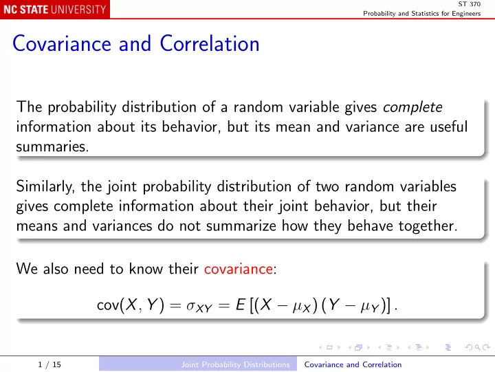
ST 370 Probability and Statistics for Engineers Covariance and Correlation The probability distribution of a random variable gives complete information about its behavior, but its mean and variance are useful summaries. Similarly, the joint probability distribution of two random variables gives complete information about their joint behavior, but their means and variances do not summarize how they behave together. We also need to know their covariance: cov( X , Y ) = σ XY = E [( X − µ X ) ( Y − µ Y )] . 1 / 15 Joint Probability Distributions Covariance and Correlation

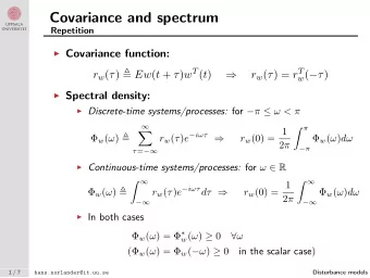
ST 370 Probability and Statistics for Engineers Example: Mobile response time x = Number of bars 1 2 3 Marginal y = Response time 4+ 0.15 0.10 0.05 0.30 3 0.02 0.10 0.05 0.17 2 0.02 0.03 0.20 0.25 1 0.01 0.02 0.25 0.28 Marginal 0.20 0.25 0.55 From the marginal distributions: µ X = 1 × 0 . 20 + 2 × 0 . 25 + 3 × 0 . 55 = 2 . 35 , µ Y = 1 × 0 . 28 + 2 × 0 . 25 + 3 × 0 . 17 + 4 × 0 . 30 = 2 . 49 . 2 / 15 Joint Probability Distributions Covariance and Correlation

ST 370 Probability and Statistics for Engineers Also from the marginal distributions, σ 2 X = 0 . 6275 , σ 2 Y = 1 . 4099 . For the covariance, we need the joint distribution: 3 4 � � σ XY = [( x − µ X ) ( y − µ Y )] f XY ( x , y ) x =1 y =1 = − 0 . 5815 . 3 / 15 Joint Probability Distributions Covariance and Correlation

ST 370 Probability and Statistics for Engineers Sign of covariance Negative covariance, as here, means that X and Y tend to move in opposite directions: a stronger signal leads to shorter response times, and conversely. Positive covariance would mean that they tend to move in the same direction; zero covariance would mean that X and Y are not linearly related. 4 / 15 Joint Probability Distributions Covariance and Correlation

ST 370 Probability and Statistics for Engineers Magnitude of covariance The magnitude of the covariance is harder to interpret; in particular, it has the units of X multiplied by the units of Y , here seconds 2 . It is easier to interpret a dimensionless quantity, the correlation coefficient cov( X , Y ) = σ XY ρ XY = . � σ X σ Y V ( X ) V ( Y ) The correlation coefficient has the same sign as the covariance, and always lies between − 1 and +1; in the example, ρ XY = − 0 . 618228. 5 / 15 Joint Probability Distributions Covariance and Correlation

ST 370 Probability and Statistics for Engineers Independence If X and Y are independent, then f XY ( x , y ) = f X ( x ) × f Y ( y ) , and � � E ( XY ) = xyf XY ( x , y ) x y � � = xyf X ( x ) f Y ( y ) x y � � = xf X ( x ) yf Y ( y ) x y = E ( X ) E ( Y ) . 6 / 15 Joint Probability Distributions Covariance and Correlation

ST 370 Probability and Statistics for Engineers More generally, E [( X − a )( Y − b )] = E ( X − a ) E ( Y − b ) and with a = µ X and b = µ Y , cov( X , Y ) = E ( X − µ X ) E ( Y − µ Y ) = 0 , and consequently also ρ XY = 0. That is, if X and Y are independent, they are also uncorrelated . The opposite is not generally true: if X and Y are uncorrelated, they might or might not be independent. 7 / 15 Joint Probability Distributions Covariance and Correlation

ST 370 Probability and Statistics for Engineers Estimating covariance and correlation The covariance σ XY and correlation ρ XY are characteristics of the joint probability distribution of X and Y , like µ X , σ X , and so on. That is, they characterize the population of values of X and Y . 8 / 15 Joint Probability Distributions Covariance and Correlation

ST 370 Probability and Statistics for Engineers From a sample of values, we estimate µ X and σ X by ¯ x and s x , the sample mean and standard deviation. By analogy with the sample variance n 1 � s 2 x ) 2 , x = ( x i − ¯ n − 1 i =1 the sample covariance is given by n 1 � s xy = ( x i − ¯ x )( y i − ¯ y ) . n − 1 i =1 9 / 15 Joint Probability Distributions Covariance and Correlation

ST 370 Probability and Statistics for Engineers The sample correlation coefficient is r xy = s xy s x s y � n i =1 ( x i − ¯ x )( y i − ¯ y ) = y ) 2 . �� n x ) 2 �� n i =1 ( x i − ¯ i =1 ( y i − ¯ Notice the similarity to the calculation of the regression coefficient � n i =1 ( x i − ¯ x )( y i − ¯ y ) = s xy = r xy × s y ˆ β 1 = . � n i =1 ( x i − ¯ x ) 2 s 2 s x x 10 / 15 Joint Probability Distributions Covariance and Correlation

ST 370 Probability and Statistics for Engineers But note the difference in context: In the regression context, we have a model Y = β 0 + β 1 x + ǫ, in which x is a fixed quantity, and Y is a random variable; In the correlation context, both X and Y are random variables. The connection between correlation and regression is deeper than just the computational similarity, but they are not the same thing. 11 / 15 Joint Probability Distributions Covariance and Correlation

ST 370 Probability and Statistics for Engineers Linear Functions of Random Variables Given random variables X 1 , X 2 , . . . , X p and constants c 1 , c 2 , . . . , c p the random variable Y given by Y = c 1 X 1 + c 2 X 2 + · · · + c p X p is a linear combination of X 1 , X 2 , . . . , X p . The expected value of Y is E ( Y ) = c 1 E ( X 1 ) + c 2 E ( X 2 ) + · · · + c p E ( X p ) 12 / 15 Joint Probability Distributions Linear Functions of Random Variables

ST 370 Probability and Statistics for Engineers The variance of Y involves both the variances and covariances of the X s. If the X s are uncorrelated, and in particular if they are independent, then V ( Y ) = c 2 1 V ( X 1 ) + c 2 2 V ( X 2 ) + · · · + c 2 p V ( X p ) . 13 / 15 Joint Probability Distributions Linear Functions of Random Variables

ST 370 Probability and Statistics for Engineers Special case: the average p , then Y is just ¯ If c 1 = c 2 = · · · = c p = 1 X , the average of X 1 , X 2 , . . . , X p If the X s all have the same expected value µ , then � ¯ � E X = µ and if they are uncorrelated and all have the same variance σ 2 , then � ¯ = σ 2 � V X p . 14 / 15 Joint Probability Distributions Linear Functions of Random Variables

ST 370 Probability and Statistics for Engineers Note that X = σ σ ¯ √ p , which becomes small when p is large. That means that when p is large, ¯ X is likely to be close to µ , a result known as the weak law of large numbers. 15 / 15 Joint Probability Distributions Linear Functions of Random Variables