Covariance and spectrum Repetition Covariance function: r w ( ) - PowerPoint PPT Presentation

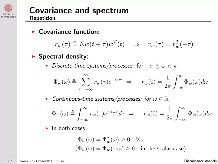
Covariance and spectrum Repetition ◮ Covariance function: r w ( τ ) � Ew ( t + τ ) w T ( t ) r w ( τ ) = r T ⇒ w ( − τ ) ◮ Spectral density: ◮ Discrete-time systems/processes: for − π ≤ ω < π � π ∞ r w (0) = 1 r w ( τ ) e − iωτ ⇒ � Φ w ( ω ) � Φ w ( ω ) dω 2 π − π τ = −∞ ◮ Continuous-time systems/processes: for ω ∈ R � ∞ � ∞ r w (0) = 1 r w ( τ ) e − iωτ dτ ⇒ Φ w ( ω ) � Φ w ( ω ) dω 2 π −∞ −∞ ◮ In both cases Φ w ( ω ) = Φ ∗ w ( ω ) ≥ 0 ∀ ω (Φ w ( ω ) = Φ w ( − ω ) ≥ 0 in the scalar case ) 1 / 7 hans.norlander@it.uu.se Disturbance models

Linear filtering and spectral factorization Repetition ◮ White noise: w ( t ) white noise ⇔ Φ w ( ω ) = R w = constant ◮ Discrete-time white noise: r w ( τ ) = 0 for all τ � = 0 ◮ Linear filtering: ◮ Discrete-time systems/processes: Φ y ( ω ) = G ( e iω )Φ u ( ω ) G ∗ ( e iω ) y ( k ) = G ( q ) u ( k ) ⇒ ◮ Continuous-time systems/processes: y ( t ) = G ( p ) u ( t ) ⇒ Φ y ( ω ) = G ( iω )Φ u ( ω ) G ∗ ( iω ) ◮ In the scalar case: Φ y ( ω ) = | G | 2 Φ u ( ω ) ◮ Spectral factorization: If 0 ≤ Φ w ( ω ) < ∞ is rational in ◮ (discrete-time:) cos ω there exists a rational G ( z ) ◮ (continuous-time:) ω 2 there exists a rational G ( s ) which is stable and minimum phase, such that Φ w ( ω ) = | G | 2 (with z = e iω / s = iω respectively). 2 / 7 hans.norlander@it.uu.se Disturbance models

State space models Discrete-time systems/processes ◮ Let v ( k ) be white noise with Ev ( k ) = 0 and r v (0) = R v . ◮ Assume that x ( k ) ∈ R n is governed by the state equation x ( k + 1) = Fx ( k ) + Gv ( k ) , with F stable. ◮ Then x ( k ) is a stationary stochastic process, and Ex ( k ) = 0 . ◮ The covariance matrix Π x = Ex ( k ) x T ( k ) = r x (0) is the solution of the discrete-time Lyapunov equation , Π x = F Π x F T + GR v G T . ◮ The covariance function of x is r x ( τ ) = Ex ( k + τ ) x T ( k ) = F τ Π x , for τ ≥ 0 . (For τ < 0 , use that r x ( τ ) = r x ( − τ ) T .) 3 / 7 hans.norlander@it.uu.se Disturbance models

State space models Continuous-time systems/processes ◮ Let v ( t ) be continuous-time white noise with Ev ( t ) = 0 and intensity R v . ◮ Assume that x ( t ) ∈ R n is governed by the state equation x ( t ) = Ax ( t ) + Bv ( t ) , ˙ with A stable. ◮ Then x ( t ) is a stationary stochastic process, and Ex ( t ) = 0 . ◮ The covariance matrix Π x = Ex ( t ) x T ( t ) is the solution of the continuous-time Lyapunov equation , 0 = A Π x + Π x A T + BR v B T . 4 / 7 hans.norlander@it.uu.se Disturbance models

Cross-covariance and cross-spectrum Some more relevant properties ◮ Consider two stationary stochastic processes, x ( t ) and y ( t ) , with Ex ( t ) = Ey ( t ) = 0 . ◮ Cross-covariance: r xy ( τ ) � Ex ( t + τ ) y T ( t ) ◮ Cross-spectrum: ∞ � r xy ( τ ) e − iωτ Φ xy ( ω ) � Discrete-time processes: τ = −∞ � ∞ Φ xy ( ω ) � r xy ( τ ) e − iωτ dτ Continuous-time processes: −∞ ◮ x ( t ) and y ( t ) independent ⇒ r xy ( τ ) ≡ 0 and Φ xy ( ω ) ≡ 0 . ◮ Discrete-time: y ( k ) = G ( q ) u ( k ) ⇒ Φ yu ( ω ) = G ( e iω )Φ u ( ω ) ◮ Continuous-time: y ( t ) = G ( p ) u ( t ) ⇒ Φ yu ( ω ) = G ( iω )Φ u ( ω ) 5 / 7 hans.norlander@it.uu.se Disturbance models

Aggregation of noise Strategy: Lump several noise sources together into one single source Let v and e be white noise of zero mean and Φ v ( ω ) = R v , Φ e ( ω ) = R e and Φ ve ( ω ) = 0 . e w y ε y v ⇔ G w G ε Σ ◮ Then Φ y ( ω ) = | G w | 2 R v + R e = rational function. ◮ By spectral factorization we get Φ y ( ω ) = | G ε | 2 for som stable, minimum phase, rational G ε ◮ ⇒ we can compute ε = G − 1 ε y (since G − 1 is stable). ε 6 / 7 hans.norlander@it.uu.se Disturbance models

The total model Incorporating the noise in the system model v 1 v 2 G w G n w n y u z G Σ ◮ u - input, ◮ z - controlled/performance variable, ◮ y - measured output, ◮ w - system/process noise, ◮ n - measurement noise, ◮ v 1 - white process noise, ◮ v 2 - white measurement noise. 7 / 7 hans.norlander@it.uu.se Disturbance models