Posterior Covariance vs. Analysis Error Covariance in Data - PowerPoint PPT Presentation
Posterior Covariance vs. Analysis Error Covariance in Data Assimilation F.-X. Le Dimet(1), I. Gejadze(2), V. Shutyaev(3) (1) Universit e de Grenoble (2)University of Strathclyde, Glasgow, UK (3) Institute of Numerical Mathematics, RAS,
Posterior Covariance vs. Analysis Error Covariance in Data Assimilation F.-X. Le Dimet(1), I. Gejadze(2), V. Shutyaev(3) (1) Universit´ e de Grenoble (2)University of Strathclyde, Glasgow, UK (3) Institute of Numerical Mathematics, RAS, Moscow, Russia ledimet@imag.fr September 27, 2013 F.-X. Le Dimet (INRIA) Posterior covariance September 27, 2013 1 / 1
Overview Introduction Analysis Error Covariance via Hessian Posterior Covariance : A Bayesian approach Effective Covariance Estimates Implementation : some remarks Asymptotic Properties Numerical Example Conclusion F.-X. Le Dimet (INRIA) Posterior covariance September 27, 2013 2 / 1
Introduction 1 There are two basic approaches for Data Assimilation: Variational Methods Kalman Filter Both lead to minimize a cost function : J ( u ) = 1 b ( u − u b ) , u − u b ) X + 1 2( V − 1 2( V − 1 ( C ϕ − y ) , C ϕ − y ) Y o , (1) o where u b ∈ X is a prior initial-value function (background state), y ∈ Y o is a prescribed function (observational data), Y o is an observation space, C : Y → Y o is a linear bounded operator. We get the same optimal solution ¯ u F.-X. Le Dimet (INRIA) Posterior covariance September 27, 2013 3 / 1
Introduction 2 u is the solution of the Optimality System : ¯ ∂ϕ � = F ( ϕ ) + f , t ∈ (0 , T ) ∂ t (2) � ϕ = u , � t =0 � ∂ϕ ∗ C ∗ V − 1 ∂ t + ( F ′ ( ϕ )) ∗ ϕ ∗ = ( C ϕ − y ) , t ∈ (0 , T ) o (3) ϕ ∗ � = 0 , � t = T V − 1 b ( u − u b ) − ϕ ∗ � t =0 = 0 (4) � F.-X. Le Dimet (INRIA) Posterior covariance September 27, 2013 4 / 1
Introduction 3 In an analysis there are two inputs: The background u b the observation y Both have error and the question is what is the impact of these errors on the analysis? The background can be considered from two different viewpoints: Variational viewpoint: the background is a regularization term in the Tykhonov’s sense to make the problem well posed Bayesian view point: the background is an a priori information on the analysis F.-X. Le Dimet (INRIA) Posterior covariance September 27, 2013 5 / 1
Introduction 4 In the linear case we get the same covariance error for the analysis : the inverse of the Hessian of the cost function. In the non linear case we get two different items: Variational approach : Analysis Error Covariance Bayesian Approach : Posterior Covariance Questions: How to compute, approximate, these elements? What are the differences? F.-X. Le Dimet (INRIA) Posterior covariance September 27, 2013 6 / 1
Analysis Error Covariance 1: True solution and Errors We assume the existence of a ”true” solution u t and an associated ”true” state ϕ t verifying: ∂ϕ t F ( ϕ t ) + f , = t ∈ (0 , T ) ∂ t ϕ t � u t . = (5) � t =0 Then the errors are defined by : u b = u t + ξ b , y = C ϕ t + ξ o with covariances V b and V o F.-X. Le Dimet (INRIA) Posterior covariance September 27, 2013 7 / 1
Analysis Error Covariance 2: Discrepancy Evolution Let δϕ = ϕ − ϕ t , δ u = u − u t . ϕ = ϕ t + τ ( ϕ − ϕ t ) , τ ∈ [0 , 1] , such that Then for regular F there exists ˜ � ∂δϕ ∂ t − F ′ ( ˜ 0 , t ∈ (0 , T ) , ϕ ) δϕ = (6) δϕ | t =0 = δ u , � ∂ϕ ∗ C ∗ V − 1 ∂ t + ( F ′ ( ϕ )) ∗ ϕ ∗ = ( C δϕ − ξ o ) , o (7) ϕ ∗ � = 0 , � t = T V − 1 b ( δ u − ξ b ) − ϕ ∗ | t =0 = 0 . (8) F.-X. Le Dimet (INRIA) Posterior covariance September 27, 2013 8 / 1
Analysis Error Covariance 3: Exact Equation for Analysis Error Let us introduce the operator R ( ϕ ) : X → Y as follows: R ( ϕ ) v = ψ, v ∈ X , (9) where ψ is the solution of the tangent linear problem ∂ψ ∂ t − F ′ ( ϕ ) ψ = 0 , ψ | t =0 = v . (10) Then, the system for errors can be represented as a single operator equation for δ u : ϕ ) δ u = V − 1 b ξ b + R ∗ ( ϕ ) C ∗ V − 1 H ( ϕ, ˜ ξ o , (11) o where ϕ ) = V − 1 + R ∗ ( ϕ ) C ∗ V − 1 H ( ϕ, ˜ CR ( ˜ ϕ ) . (12) o b F.-X. Le Dimet (INRIA) Posterior covariance September 27, 2013 9 / 1
Analysis Error Covariance 4 : H Operator The operator H ( ϕ, ˜ ϕ ) : X → X can be defined by ∂ψ ∂ t − F ′ ( ˜ ϕ ) ψ = 0 , ψ | t =0 = v , (13) − ∂ψ ∗ ∂ t − ( F ′ ( ϕ )) ∗ ψ ∗ = − C ∗ V − 1 C ψ, ψ ∗ � t = T = 0 , (14) o � ϕ ) v = V − 1 b v − ψ ∗ | t =0 . H ( ϕ, ˜ (15) The operator H ( ϕ, ˜ ϕ ) is neither symmetric, nor positive definite. ϕ = ˜ ϕ = θ , it becomes the Hessian H ( θ ) of the cost function J 1 in the following auxiliary DA problem: find δ u and δϕ such that J 1 ( δ u ) = inf v J 1 ( v ), where J 1 ( δ u ) = 1 b ( δ u − ξ b ) , δ u − ξ b ) X + 1 2( V − 1 2( V − 1 ( C δϕ − ξ o ) , C δϕ − ξ o ) Y o , o (16) and δϕ satisfies the problem ∂δϕ ∂ t − F ′ ( θ ) δϕ = 0 , δϕ � t =0 = δ u . (17) � F.-X. Le Dimet (INRIA) Posterior covariance September 27, 2013 10 / 1
Analysis Error Covariance 5 : Analysis Error Covariance via Hessian The optimal solution (analysis) error δ u is assumed to be unbiased, i.e. E [ δ u ] = 0, and V δ u · = E [( · , δ u ) X δ u ] = E [( · , u − u t ) X ( u − u t )] . (18) ϕ independent of ξ o , ξ b is apparently ϕ t and using The best value of ϕ and ˜ ϕ ) ≈ R ( ϕ t ) , R ∗ ( ϕ ) ≈ R ∗ ( ϕ t ) , R ( ˜ (19) the error equation reduces to H ( ϕ t ) δ u = V − 1 b ξ b + R ∗ ( ϕ t ) C ∗ V − 1 ξ o , H ( · ) = V − 1 + R ∗ ( · ) C ∗ V − 1 CR ( · ) . o o b (20) We express δ u from equation ( ?? ) δ u = H − 1 ( ϕ t )( V − 1 b ξ b + R ∗ ( ϕ t ) C ∗ V − 1 ξ o ) o and obtain for the analysis error covariance V δ u = H − 1 ( ϕ t )( V − 1 + R ∗ ( ϕ t ) C ∗ V − 1 CR ( ϕ t )) H − 1 ( ϕ t ) = H − 1 ( ϕ t ) . (21) b o F.-X. Le Dimet (INRIA) Posterior covariance September 27, 2013 11 / 1
Analysis Error Covariance 6 : Approximations In practice the ’true’ field ϕ t is not known, thus we have to use an approximation ¯ ϕ associated to a certain optimal solution ¯ u defined by the real data (¯ u b , ¯ y ), i.e. we use V δ u = H − 1 ( ¯ ϕ ) . (22) In (Rabier and Courtier,1992), the error equation is derived in the form ( V − 1 + R ∗ ( ϕ ) C ∗ V − 1 CR ( ϕ )) δ u = V − 1 b ξ b + R ∗ ( ϕ ) C ∗ V − 1 ξ o . (23) b o o ϕ ) → R ( ϕ t ) and R ∗ ( ϕ ) → R ∗ ( ϕ t ); we call The error due to transitions R ( ˜ ϕ instead of ϕ t in the Hessian it the ’linearization’ error. The use of ¯ computations leads to another error, which shall be called the ’origin’ error. F.-X. Le Dimet (INRIA) Posterior covariance September 27, 2013 12 / 1
Posterior Covariance : Bayesian Approach 1 Given u b ∼ N (¯ u b , V b ), y ∼ N (¯ y , V o ), the following expression for the posterior distribution of u is derived from the Bayes theorem: y ) = C · exp ( − 1 2( V − 1 p ( u | ¯ b ( u − ¯ u b ) , u − ¯ u b ) X ) · exp( − 1 2( V − 1 ( C ϕ − ¯ y ) , C ϕ − ¯ y ) Y o ) . o (24) The solution to the variational DA problem with the data y = ¯ y and u b = ¯ u is equal to the mode of p ( u , ¯ y ) (see e.g. Lorenc, 1986; Tarantola, 1987). Accordingly, the Bayesian posterior covariance is defined by : V δ u · = E [( · , u − E [ u ]) X ( u − E [ u ]) (25) with u ∼ p ( u | ¯ y ). F.-X. Le Dimet (INRIA) Posterior covariance September 27, 2013 13 / 1
Posterior Covariance : Bayesian Approach 2 In order to compute V δ u by the Monte Carlo method, one must generate a sample of pseudo-random realizations u i from p ( u | ¯ y ). We will consider u i to be the solutions to the DA problem with the perturbed data y + ξ o , where ξ b ∼ N (0 , V b ), ξ o ∼ N (0 , V o ). u b = ¯ u b + ξ b , and y = ¯ Further we assume that E [ u ] = ¯ u , where ¯ u is the solution to the unperturbed problem in which case V δ u can be approximated as follows V δ u · = E [( · , u − ¯ u ) X ( u − ¯ u )] = E [( · , δ u ) X δ u ] . (26) F.-X. Le Dimet (INRIA) Posterior covariance September 27, 2013 14 / 1
Posterior Covariance : O.S. for Errors Unperturbed O.S. with u b = ¯ u b , y = ¯ y : ∂ ¯ ϕ � ∂ t = F ( ¯ ϕ ) + f , ϕ t =0 = ¯ u , (27) � ϕ ∗ ∂ ¯ ϕ )) ∗ ¯ ϕ ∗ = C ∗ V − 1 ∂ t + ( F ′ ( ¯ ϕ ∗ � ( C ¯ ϕ − ¯ y ) , ¯ t = T = 0 , (28) o � V − 1 ϕ ∗ � b (¯ u − ¯ u b ) − ¯ t =0 = 0 (29) � With perturbations : u b = ¯ u b + ξ b , y = ¯ y + ξ o , where ξ b ∈ X , ξ o ∈ Y o . ϕ , δϕ ∗ = ϕ ∗ − ¯ δ u = u − ¯ u , δϕ = ϕ − ¯ ϕ ∗ . ∂δϕ � = F ( ϕ ) − F ( ¯ ϕ ) , δϕ t =0 = δ u , (30) � ∂ t ∂δϕ ∗ +( F ′ ( ϕ )) ∗ δϕ ∗ = [(( F ′ ( ¯ ϕ ∗ + C ∗ V − 1 ϕ )) ∗ − F ′ ( ϕ )) ∗ ] ¯ ( C δϕ − ξ o ) , (31) o ∂ t V − 1 b ( δ u − ξ b ) − δϕ ∗ � t =0 = 0 . (32) � F.-X. Le Dimet (INRIA) Posterior covariance September 27, 2013 15 / 1
Recommend
More recommend
Explore More Topics
Stay informed with curated content and fresh updates.
