Probability Distribution 1. Probability Distribution: ( ,..., ) - PDF document

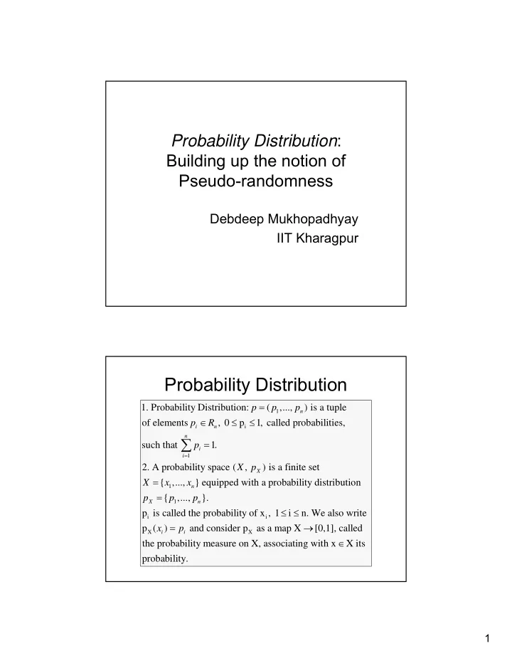
Probability Distribution : Building up the notion of Pseudo-randomness Debdeep Mukhopadhyay IIT Kharagpur Probability Distribution  1. Probability Distribution: ( ,..., ) is a tuple p p p 1 n    of elements , 0 p 1, called probabilities, p R i n i n   such that 1. p i  i 1 2. A probability space ( , ) is a finite set X p X  X { ,..., x x } equipped with a probability distribution 1 n  { ,..., }. p p p X 1 n   p is called the probability of x , 1 i n. We also write i i   p ( ) and consider p as a map X [0,1], called x p X X i i  the probability measure on X, associating with x X its probability. 1

 3. An event in a probability space (X,p ) is a subset X  of X.    p ( ) ( ) p y X X   y   p ( ) 1 X X A probability space X is the model of a random experiment. n independent repetitions of the random experiment are modeled     n by the direct product: X ... X X X Some interesting results…   Let be an event in a probability space X, with Pr[ ]=p>0. Repeatedly, we perform the random experiment X independently. Let, G be the expected number of experiments 1  of X, until occurs the first ti me. Prove that: E(G)= p   d d 1 1                1 1 Pr[ ] (1 ) t ( ) (1 ) t (1 ) =-p t ( 1) . G t p p E G tp p p p dp dp p p   1 1 t t 2

Another Useful result Let R, S and B be jointly distributed r.v with values in {0,1}. Assume that B and S are independent and that B is uniformly distributed: Pr(B=0)=Pr(B=1)=1/2 Prove that: Pr(R=S)=1/2 + Pr(R=B|S=B)-Pr(R=B) Pr(S=B)=Pr(S=0)Pr(B=0|S=0)+Pr(S=1)Pr(B=1|S=1) =Pr(S=0)Pr(B=0)+Pr(S=1)Pr(B=1) 1 1 = (Pr(S=0)+Pr(S=1))= 2 2 1   Likewise ,Pr( S B ) 2 1 1        Pr( R S ) Pr( R B S | B ) Pr( R B S | B ) 2 2 1 1       = [P r( | ) 1 Pr( | )] R B S B R B S B 2 2  1 1 Pr[(R=B) (S=B)]     = [Pr( R B S | B ) ]  2 2 Pr( ) S B       (R=B)=((R=B) (S=B)) (( ) ( )) R B S B         Pr[ R B ] Pr[(R=B) (S=B)] Pr[( R B ) ( S B )]      1 1 Pr[ ] Pr[( ) ( )] ) R B R B S B        Pr( ) (Pr( | ) R S R B S B  2 2 Pr( S B )      1 1 Pr[ ] Pr[ ]Pr[( ) | ( )] R B S B R B S B      (Pr( | ) ) R B S B 2 2 1/ 2     1 1 Pr[ R B ] 1/ 2Pr[( R B ) | ( S B )]     = (Pr( | ) ) R B S B 2 2 1/ 2 1      = Pr( R B S | B ) Pr[ R B ] 2 3

Statistical Distance between Probability Distributions  Let p and p be probability distributions on a finite set X.  The statistical distance between p and p is: 1      dist(p,p) | ( ) p( ) | x X p x x  2 The statistical distance between probability distributions p  and p on a finite set X is the maximal distance between the probabilities of events in X, ie.       dist(p,p) max | ( ) ( )| p p   X The events in X are the subsets of X. We divide the subsets into three categories:      { x X | p x ( ) p x ( )} 1      { | ( ) ( )} x X p x p x 2      { | ( ) ( )} x X p x p x 3 3        We have 0=p(X)-p( X ) [p( ) p ( )] i i i=1                  p( ) p ( ) 0 p( ) p ( ) (p( ) p ( )) 3 3 1 1 2 2  Now because of the definition of , 1              max |p( )-p( )|= p( ) ( ) (p( ) ( )) p p   X 1 1 2 2 1       dist(p,p) | ( ) p( ) | p x x  2 x X 1         ( [ ( ) p( )] [ ( ) p( )]) p x x p x x     2 x x 1 2 1               = [(p( ) ( )) (p( ) ( ))] max | ( ) ( )| p p p p   1 1 2 2 X 2 4

Indistinguishable Distributions   p and p are called polynomially close or -indistinguishable if: 1     dist(p,p) ( ) n ( ) P n  where ( ) is a negligible quantity. p(n) is a polynomial in n. n Pseudo-random sequence: No efficient observer can distinguish it from a uniformly chosen string of the same length. This approach leads to the concept of pseudo- random generators, which is a fundamental concept with lot of applications. Proof    Let J { | , , are primes,|r|=|s|=k,r s} and n n rs r s k   * x Z and x Z are polynomially close. Is the result n n dependent on the choice of r and s? 5

Pseudorandom Bit Generator • Let I=(I n ) n Є N be a key set with security parameter n, and let K be a probabilistic sampling algorithm for I, which on input (n) outputs an i Є I n . Let l be a polynomial function in the security parameter. • A pseudorandom bit generator with key generator K and stretch function l is a family of functions G=(G i ) i Є I of functions. – G i : X i  {0,1} l(n) , i Є I(n) – G is computable by a deterministic polynomial algorithm G. • G(i,x)=G i (x) for all i Є I and x Є X i • there is a uniform sampling algorithm for X. On input i, it outputs x Є X i . Pseudorandom Bit Generator    ( ) n l n | Pr( ( , ) 1: (1 ), {0,1} A i z i K z       n Pr ( , ( ) 1) : (1 ), | A i G x i K x X i i 1  ( ) P n 6

x B i f i f i (x) B i f i f i (f i (x)) B i Q(k)-1 (x) f i B i If the discrete log assumption is true,    * x ( : , mod ) Exp Exp Z Z x g p  , 1 p g p p  * with I={(p,g)|p is prime, g Z a primitive root} p is a bijective one-way function.   0 for 0 x<(p-1)/2   MSB ( ) x   p  1 for (p-1)/2 x p-1 i s a hard-core predicate for Exp. Exp can be treated as a one-way permutation, * identifying Z with Z . p-1 p    Z {0,..., p 2} p 1   * {1,..., 1} Z p p    using the mapping 0 p-1, 1 1, ...,p-2 p-2 Induced PRG is a called B lum Micali Generator. 7

Blum-Micali-Yao’s Theorem • Suppose f is a length preserving one-way function. Let B be a hard core predicate for f. Then the algorithm G defined by G(x)=F(x)||B(x)=F(x).B(x) is a pseudo random generator. Let D be an algorithm distinguishing between G(U ) and U . n n+1       Pr[ ( ( )) 1] Pr[ ( ) 1] D G U D U  n n 1  (1) : E [ ( ). ( )] Define f U b U n n  (2) E [ ( ). ( )] f U b U n n   (1) : ( ) ( ). ( ) E Note G U f U b U n n n 8

 ,Pr[ ( ) 1] Also D U  n 1   Pr[ ( ( ). ) 1][ , is bijective] D f U U as f n 1    Pr[ ( ( ). ( )) 1]Pr[ ( ) ] D f U b U b U U n n n 1    Pr[ ( ( ). ( )) 1]Pr[ ( ) ] D f U b U b U U n n n 1 1 (Pr[     ( ( ). ( )) 1] Pr[ ( ( ). ( )) 1]) D f U b U D f U b U n n n n 2 1 (Pr[     (1) (2) (E ) 1] Pr[ ( E ) 1]) D D 2     Pr[ ( ( )) 1] Pr[ ( ) 1] D G U D U  n n 1 1       (1) (1) (2) Pr[ ( 1] (Pr[ (E ) 1] Pr[ ( E ) 1]) D E D D 2 1 (Pr[       (1) (2) ( 1] Pr[ ( E ) 1]) D E D 2 9

Thus using D if we make an algorithm to guess the hardcore predicate B(.) from y=f(x), then we are done. Algorithm A:  1. Select uniformly in {0,1}     2. If D(y. ) 1, output , else 1- What is the probability that A is able to compute the hardcore predicate?: Pr[A(f(X)=b(X)]=Pr[A(f(U )=b(U )] n n  =Pr[D(f(U )U )=1 U =b(U )] n 1 1 n  +Pr[D(f(U )U )=0 1-U =b(U )] n 1 1 n 1 = (Pr[D(f(U )b(U ))=1] n n 2 +Pr[D(f(U )b (U ))=0]) n n 1 = (Pr[D(f(U )b(U ))=1] n n 2 1  + (1 Pr[D(f(U )b(U )]=1) n n 2 1 1  = (Pr[D(f(U )b(U ))=1]-Pr[D(f(U )b(U )]=1) n n n n 2 2 1 1     (1) (2) = (Pr[ D E ( 1] Pr[ D ( E ) 1]) 2 2 1    . Thus we reach a contradiction. 2 10

Let I=(I ) be a key set with security parameter k,  k k N   and let Q Z[X] be a positive polynomial. Let f=(f : ) D D  i i i i I be a family of one-way permutations with hard core predicate  B=(B : {0,1}) and ke y generator K. Let G=G(f,B,Q) D  i i i I be the induced pseudorandom bit generator. Is this a PR Bit Generator? x B i f i f i (x) B i f i f i (f i (x)) B i Q(k)-1 (x) f i B i 11