Changing the probability distribution Recall the binary tree with a - PowerPoint PPT Presentation

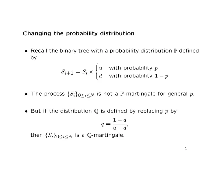
Changing the probability distribution • Recall the binary tree with a probability distribution P defined by  with probability p u  S i +1 = S i × with probability 1 − p d  • The process { S i } 0 ≤ i ≤ N is not a P -martingale for general p . • But if the distribution Q is defined by replacing p by q = 1 − d u − d, then { S i } 0 ≤ i ≤ N is a Q -martingale. 1

• Consider a path with N ( i ) up-steps in the first i steps, so S i = S 0 u N ( i ) d i − N ( i ) . • Its probability under P is p N ( i ) (1 − p ) i − N ( i ) and under Q is q N ( i ) (1 − q ) i − N ( i ) = L i × p N ( i ) (1 − p ) i − N ( i ) where � N ( i ) � � i − N ( i ) � 1 − q q L i = 1 − p p 2

• Notice that for a given i , L i depends on the path up to time iδt , and is therefore a random variable; it is also F i - measurable. • So { L i } 0 ≤ i ≤ N is an adapted stochastic process. • { L i } 0 ≤ i ≤ N is also: – positive, with P -probability 1; – a P -martingale (needs proof!); – with expected value 1. 3

• Also, if C is F N -measurable, such as a claim with maturity Nδt , then E Q [ C ] = E P [ L N C ] . • L i is the Radon-Nikodym derivative of Q with respect to P on F i : L i = d Q � � . � d P � F i • The measure Q , equivalent to P , under which { S i } 0 ≤ i ≤ N is a martingale, i.e. the equivalent martingale measure , is defined by the process { L i } 0 ≤ i ≤ N . 4

Girsanov’s Theorem • Suppose that { W t } t ≥ 0 is a P -Brownian motion with the nat- ural filtration {F t } t ≥ 0 and that { θ t } t ≥ 0 is an {F t } t ≥ 0 -adapted process such that for a given T > 0 � T � � �� 1 0 θ 2 exp < ∞ E t dt 2 • Define � t � t 0 θ s dW s − 1 � � 0 θ 2 L t = exp − s ds 2 5

� � • Note that { L t } 0 ≤ t ≤ T is a positive P , {F t } 0 ≤ t ≤ T -martingale with expected value 1. • Let P ( L ) be the measure on F T defined by � P ( L ) ( A ) = E [ 1 A L T ] = A L T ( ω ) P ( dω ) . • Then under P ( L ) , the process { W ( L ) } 0 ≤ t ≤ T defined by t � t W ( L ) = W t + 0 θ s ds t is a standard Brownian motion. 6

• Note that dW ( L ) = dW t + θ t dt, t so under P , { W ( L ) } 0 ≤ t ≤ T has non-zero drift, and is not a t standard Brownian motion. • Expected values: if φ t is F t -measurable, then E P ( L ) [ φ t ] = E [ φ t L t ] and more generally, for 0 ≤ s < t , L t � � � E P ( L ) [ φ t | F s ] = E � φ t � F s � L s 7

Brownian Martingale Representation Theorem � � • As always, Ω , F , {F t } t ≥ 0 , P is a filtered probability space, � � and { W t } t ≥ 0 is a P , {F t } t ≥ 0 -Brownian motion. • Recall that if { f t } t ≥ 0 is predictable and square-integrable (strictly, f ∈ H T ), then � t M t = 0 f s dW s � � is a P , {F t } t ≥ 0 -martingale. 8

• A partial converse exists: suppose that {F t } t ≥ 0 is the natural filtration of { W t } t ≥ 0 . • Representation Theorem: if, on the same filtered probability � � space, { M t } t ≥ 0 is a square-integrable continuous P , {F t } t ≥ 0 - martingale, then there exists a predictable process { θ t } t ≥ 0 such that � t M t − M 0 = 0 θ s dW s with probability 1. • That is, every continuous square-integrable martingale is a stochastic integral with respect to Brownian motion. 9

• In some cases, we do not need to assume the existence of the Brownian motion; instead, we can construct it: • If [ M ] t is almost surely absolutely continuous, with = d [ M ] t △ > 0 λ t dt with probability 1, we can define � t 1 ˜ W t = √ λ s dM s . 0 10

� � • Then { ˜ W t } t ≥ 0 is a -martingale, and P , {F t } t ≥ 0 � 2 � 2 � � 1 1 d [ ˜ W ] t = √ λ t d [ M ] t = √ λ t λ t dt = dt. � � • So { ˜ W t } t ≥ 0 is a P , {F t } t ≥ 0 -Brownian motion, and � t √ λ s d ˜ M t − M 0 = W s . 0 11

Feynman-Kac Representation • The probabilistic approach to assigning a value to a contin- gent claim is: – Find a measure Q under which the discounted price of the underlying asset is a martingale; – The value of the claim at time t is its discounted expected value under Q , conditional on F t . • The value also satisfies a partial differential equation, and may be found by solving it. 12

• Assume that the function F solves the boundary value prob- lem 2 σ ( t, x ) 2 ∂ 2 F ∂x ( t, x ) + 1 ∂F ∂t ( t, x ) + µ ( t, x ) ∂F ∂x 2 ( t, x ) = 0 , for 0 ≤ t < T , and F ( T, x ) = Φ( x ) . • Define { X t } 0 ≤ t ≤ T to be the solution of the stochastic differ- ential equation dX t = µ ( t, X t ) dt + σ ( t, X t ) dW t , 0 ≤ t ≤ T, where { W t } t ≥ 0 is standard Brownian motion under the prob- ability measure P . 13

• If � T � 2 � �� σ ( t, X t ) ∂F ∂x ( t, X t ) dt < ∞ , 0 E then F ( t, x ) = E P [Φ( X T ) | X t = x ] . • Black and Scholes originally derived their expression for the price of a European option by solving the corresponding pde. 14